Quick Guide

Of course, follow the installation instructions first. A complete working example is shown below, and in the section that follows each command is described in detail.

Basic example

Here we show the input file required for the study of the solvation of a protein by the TMAO solvent, which is a molecule 4 atoms. The protein is assumed to be at infinite dilution in the simulation. The trajectory of the simulation is in DCD format in this example, which is the default output of NAMD and CHARMM simulation packages.

Input files

The files necessary to run this would be:

system.pdb: a PDB file of the complete simulated system.
trajectory.dcd: the simulation trajectory, here exemplified in the DCD format.
script.jl: the Julia script, described below.

These files are not provided for this example. For complete running examples, please check our examples section.

The Julia script

# Activate environment (see the Installation -> Recommended Workflow manual section)
import Pkg;
Pkg.activate(".");

# Load packages
using ComplexMixtures
using PDBTools
using Plots

# Load PDB file of the system
atoms = readPDB("./system.pdb")

# Select the protein and the TMAO molecules
protein = select(atoms, "protein")
tmao = select(atoms, "resname TMAO")

# Setup solute and solvent structures. We need to provide
# either the number of atoms per molecule, or the number
# of molecules in each selection.
solute = AtomSelection(protein, nmols=1)
solvent = AtomSelection(tmao, natomspermol=14)

# Setup the Trajectory structure: this will define which
# coordinates are used to compute the MDDF when reading
# the trajectory file.
trajectory = Trajectory("./trajectory.dcd", solute, solvent)

# Run the calculation and get results: this is the computationally
# intensive part of the calculation.
results = mddf(trajectory, Options(bulk_range=(8.0, 12.0)))

# Save the results to recover them later if required
save(results, "./results.json")

# Plot the some of the most important results.
#
# - The results.d array contains the distances. 
# - The results.mddf array contains the MDDF.
# - The results.kb array contains the Kirkwood-Buff integrals.
#
plot(results.d, results.mddf, xlabel="d / Å", ylabel="MDDF") # plot the MDDF
savefig("./mddf.pdf")
plot(results.d, results.kb, xlabel="d / Å", ylabel="KB / cm³ mol⁻¹") # plot the KB 
savefig("./kb.pdf")

Given that this code is saved into a file named script.jl, it can be run within the Julia REPL with:

julia> include("script.jl")

or directly with:

julia -t auto script.jl

where -t auto will launch julia with multi-threading. It is highly recommended to use multi-threading!

Note

Some newer CPUs have "fast" and "slow" cores, designed for performance or energy savings. Thus using all cores, with -t auto, may not be the best strategy for optimal performance. Experimenting with different number of cores using -t N where N is the number of cores used is always necessary for tunning performance.

Detailed description of the example

Start julia and load the ComplexMixtures package, using:

using ComplexMixtures

And here we will use the PDBTools package to obtain the selections of the solute and solvent molecules:

using PDBTools

(see Set solute and solvent for details).

The fastest way to understand how to use this package is through an example.

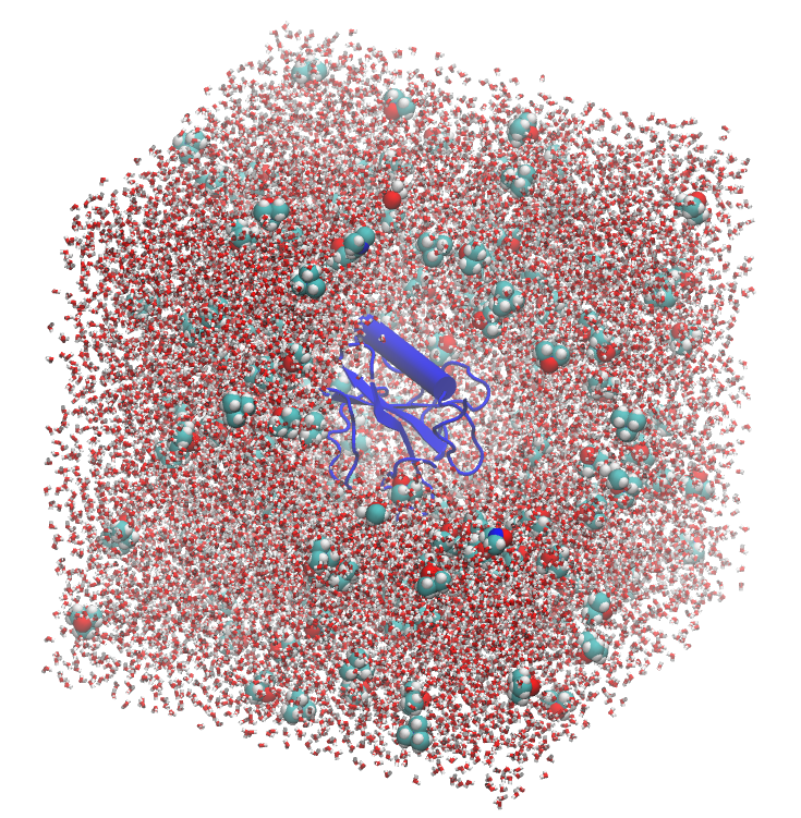
Let us consider a system of three components: a protein, water, a cosolvent: TMAO (trimetylamine-N-oxyde), which is a common osmolyte known to stabilize protein structures. A picture of this system is shown below, with the protein in blue, water, and TMAO molecules. The system was constructed with Packmol and the figure was produced with VMD.

We want to study the interactions of the protein with TMAO in this example. The computation of the MDDF is performed by defining the solute and solvent selections, and running the calculation on the trajectory.

Define the protein as the solute

To define the protein as the solute, we will use the PDBTools package, which provides a handy selection syntax. First, read the PDB file using

atoms = readPDB("./system.pdb")

Then, let us select the protein atoms (here we are using the PDBTools.select function):

protein = select(atoms, "protein")

And, finally, let us use the AtomSelection function to setup the structure required by the MDDF calculation:

solute = AtomSelection(protein, nmols=1)

Note

It is necessary to indicate how many molecules (in this case, nmols=1, so that ComplexMixtures knows that the solute is to be considered as single structure. In this case there is no ambiguity, but if the solute was a micelle, for example, this option would let ComplexMixtures know that one wants to consider the micelle as a single structure.

Define TMAO the solvent to be considered

Equivalently, the solvent is set up with:

tmao = select(atoms, "resname TMAO")
solvent = AtomSelection(tmao, natomspermol=14)

Note

Here we opted to provide the number of atoms of a TMAO molecules (with the natomspermol keyword). This is generally more practical for small molecules than to provide the number of molecules.

Set the Trajectory structure

The solute and solvent data structures are then fed into the Trajectory data structure, together with the trajectory file name, with:

trajectory = Trajectory("trajectory.dcd", solute, solvent)

In the case, the trajectory is of NAMD "DCD" format. All formats supported by Chemfiles are automatically recognized.

Finally, run the computation and get the results:

If default options are used (as the bin size of the histograms, read all frames without skipping any), just run the mddf with:

results = mddf(trajectory, Options(bulk_range=(8.0, 12.0)))

Some optional parameters for the computation are available in the Options section. Depending on the number of atoms and trajectory length, this can take a while. Computing a MDDF is much more expensive than computing a regular radial distribution function, because the normalization requires the generation of an ideal distribution of the molecules in the system.

The `results` data structure obtained

The results data structure contains all the results of the MDDF calculation, including:

results.d : Vector containing the distances to the solute.

results.mddf : Vector containing the minimum-distance distribution function at each distance.

That means, for example, that

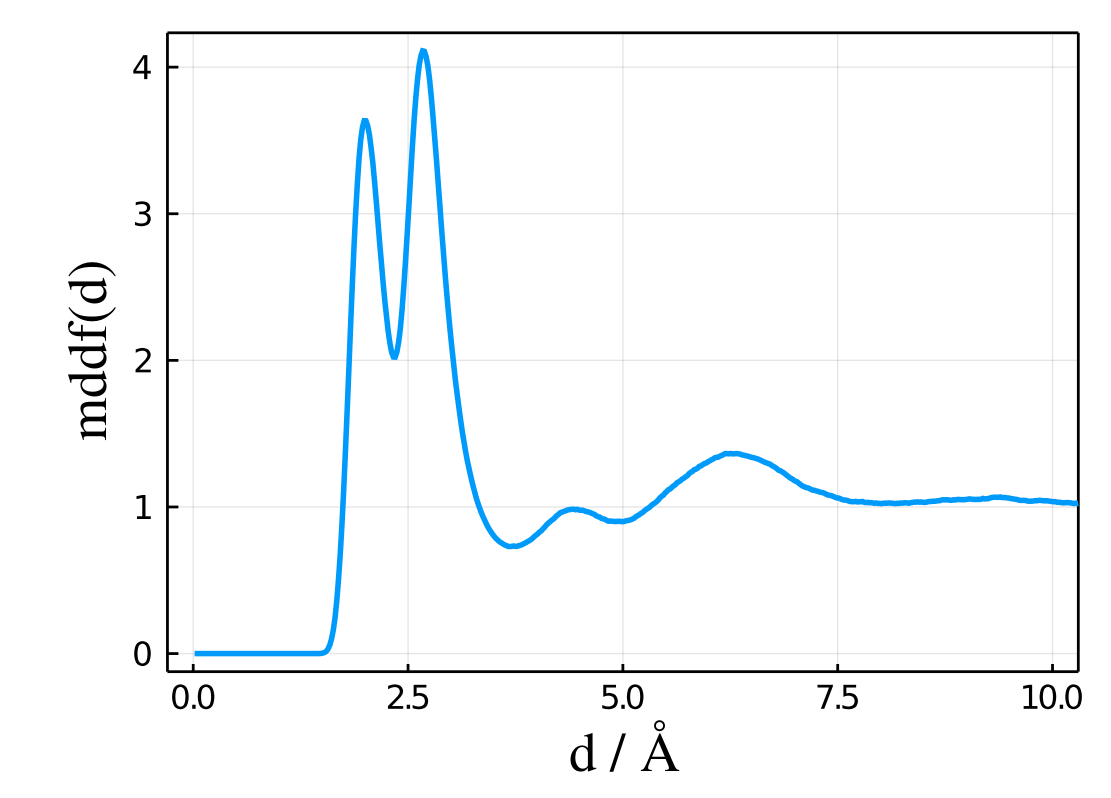
plot(results.d, results.mddf, xlabel="d / Å", ylabel="mddf(d)")

results in the expected plot of the MDDF of TMAO as a function of the distance to the protein:

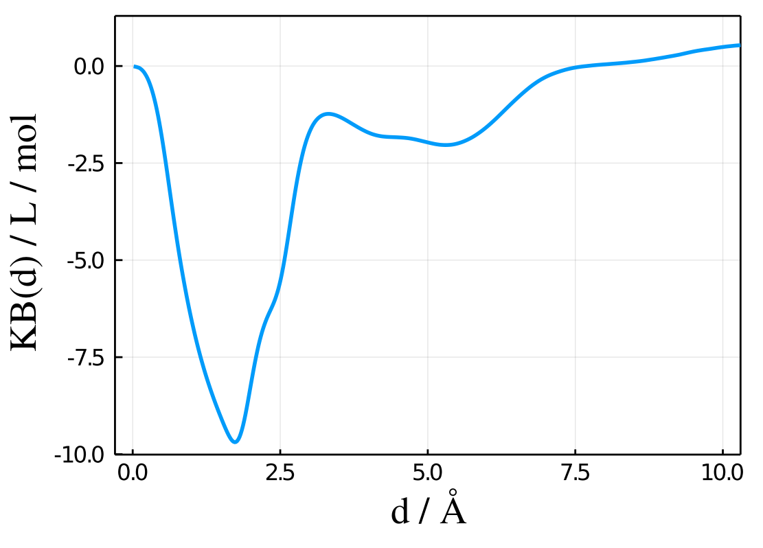
The Kirkwood-Buff integral corresponding to that distribution is provided in the results.kb vector, and can be also directly plotted with

plot(results.d, results.kb, xlabel="d / Å", ylabel="KB(d) / L / mol")

to obtain:

See the Atomic and group contributions section for a detailed account on how to obtain a molecular picture of the solvation by splitting the MDDF in the contributions of each type of atom of the solvent, each type of residue of the protein, etc.

Save the results

The results can be saved into a file (with JSON format) with:

save(results, "./results.json")

And these results can be loaded afterwards with:

load("./results.json")

Alternatively, a human-readable set of output files can be obtained to be analyzed in other software (or plotted with alternative tools), with

write(results,"./results.dat")