Protein in water/glycerol

The following examples consider a system composed a protein solvated by a mixture of water and glycerol, built with Packmol. The simulations were performed with NAMD with periodic boundary conditions and a NPT ensemble at room temperature and pressure. Molecular pictures were produced with VMD and plots were produced with Julia's Plots library.

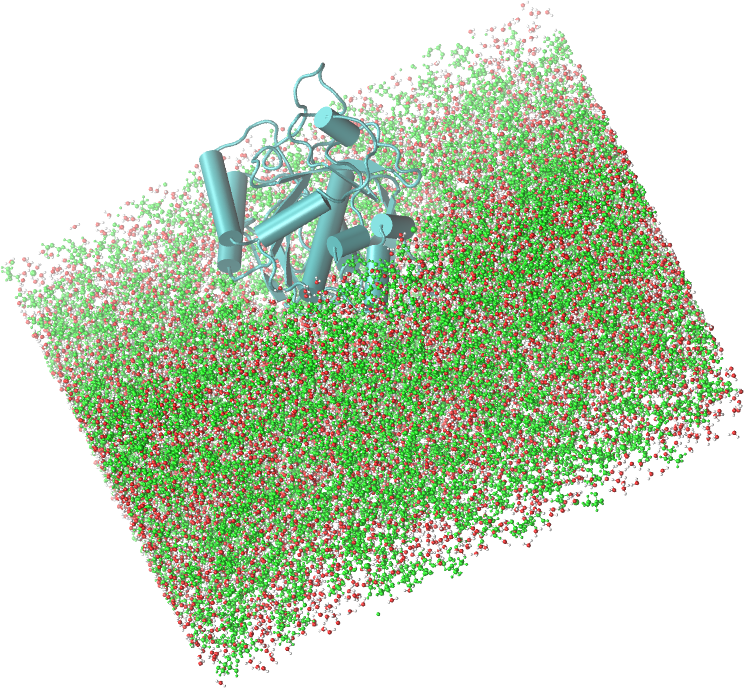
Image of the system of the example: a protein solvated by a mixture of glycreol (green) and water, at a concentration of 50%vv.

Index

• Data, packages, and execution
• MDDF, KB integrals, and group contributions
• 2D density map
• 3D density map

Data, packages, and execution

The files required to run this example are:

• system.pdb: The PDB file of the complete system.
• glyc50_traj.dcd: Trajectory file. This is a 1GB file, necessary for running from scratch the calculations.

To run the scripts, we suggest the following procedure:

1. Create a directory, for example example1.
2. Copy the required data files above to this directory.
3. Launch julia in that directory, activate the directory environment, and install the required packages. This is done by launching Julia and executing:

   import Pkg 
   Pkg.activate(".")
   Pkg.add(["ComplexMixtures", "PDBTools", "Plots", "LaTeXStrings", "EasyFit"])
   exit()

4. Copy the code of each script in to a file, and execute with:

   julia -t auto script.jl

   Alternativelly (and perhaps preferrably), copy line by line the content of the script into the Julia REPL, to follow each step of the calculation. For a more advanced Julia usage, we suggest the VSCode IDE with the Julia Language Support extension.

MDDF, KB integrals, and group contributions

Here we compute the minimum-distance distribution function, the Kirkwood-Buff integral, and the atomic contributions of the solvent to the density. This example illustrates the regular usage of ComplexMixtures, to compute the minimum distance distribution function, KB-integrals and group contributions.

# Activate environment in current directory
import Pkg;
Pkg.activate(".");

# Run this once, to install necessary packages:
# Pkg.add(["ComplexMixtures", "PDBTools", "Plots", "LaTeXStrings"])

# Load packages
using ComplexMixtures
using PDBTools
using Plots, Plots.Measures
using LaTeXStrings

# The complete trajectory file can be downloaded from (1Gb):
# https://www.dropbox.com/scl/fi/zfq4o21dkttobg2pqd41m/glyc50_traj.dcd?rlkey=el3k6t0fx6w5yiqktyx96gzg6&dl=0

# The example output file is available at:
# 
# Load PDB file of the system
atoms = readPDB("./system.pdb")

# Select the protein and the GLYC molecules
protein = select(atoms, "protein")
glyc = select(atoms, "resname GLYC")

# Setup solute and solvent structures
solute = AtomSelection(protein, nmols=1)
solvent = AtomSelection(glyc, natomspermol=14)

# Path to the trajectory file
trajectory_file = "./glyc50_traj.dcd"

# Run mddf calculation, and save results
trajectory = Trajectory(trajectory_file, solute, solvent)
results = mddf(trajectory, Options(bulk_range=(10.0, 15.0)))
save(results, "glyc50_results.json")
println("Results saved to glyc50_results.json")

#
# Produce plots
#
# Default options for plots 
Plots.default(
    fontfamily="Computer Modern",
    linewidth=2,
    framestyle=:box,
    label=nothing,
    grid=false
)

#
# The complete MDDF and the Kirkwood-Buff Integral
#
plot(layout=(1, 2))
# plot mddf
plot!(results.d, results.mddf,
    xlabel=L"r/\AA",
    ylabel="mddf",
    subplot=1
)
hline!([1], linestyle=:dash, linecolor=:gray, subplot=1)
# plot KB integral
plot!(results.d, results.kb / 1000, #to L/mol
    xlabel=L"r/\AA",
    ylabel=L"G_{us}/\mathrm{L~mol^{-1}}",
    subplot=2
)
# size and margin
plot!(size=(800, 300), margin=4mm)
savefig("./mddf.png")
println("Created plot mddf.png")

#
# Atomic contributions to the MDDF
#
hydroxyls = ["O1", "O2", "O3", "H1", "H2", "H3"]
aliphatic = ["C1", "C2", "HA", "HB", "HC", "HD"]
hydr_contrib = contributions(results, SolventGroup(hydroxyls))
aliph_contrib = contributions(results, SolventGroup(aliphatic))

plot(results.d, results.mddf,
    xlabel=L"r/\AA",
    ylabel="mddf",
    size=(600, 400)
)
plot!(results.d, hydr_contrib, label="Hydroxyls")
plot!(results.d, aliph_contrib, label="Aliphatic chain")
hline!([1], linestyle=:dash, linecolor=:gray)
savefig("./mddf_atom_contrib.png")
println("Created plot mddf_atom_contrib.png")

Output

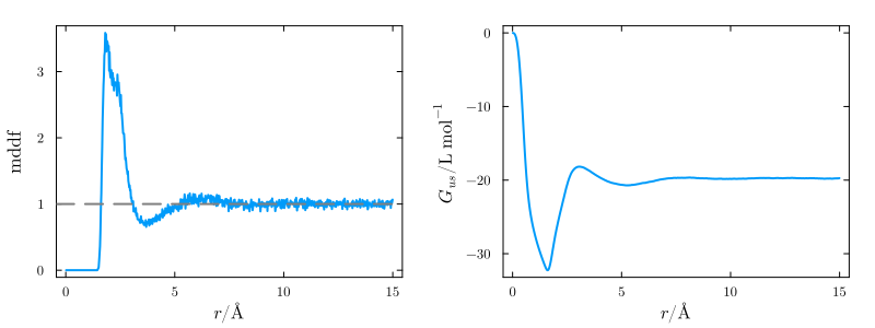
The code above will produce the following plots, which contain the minimum-distance distribution of glycerol relative to the protein, and the corresponding KB integral:

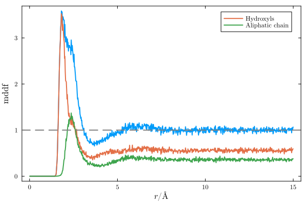
and the same distribution function, decomposed into the contributions of the hydroxyl and aliphatic groups of glycerol:

options = Options(bulk_range=(10.0, 15.0), stride=5)
mddf(trajectory, options)

2D density map

In this followup from the example aboave, we compute group contributions of the solute (the protein) to the MDDFs, split into the contributions each protein residue. This allows the observation of the penetration of the solvent on the structure, and the strength of the interaction of the solvent, or cossolvent, with each type of residue in the structure.

# Activate environment in current directory
import Pkg;
Pkg.activate(".");

# Run this once, to install necessary packages:
# Pkg.add(["ComplexMixtures", "PDBTools", "Plots", "LaTeXStrings"])

# Load packages
using ComplexMixtures
using PDBTools
using Plots, Plots.Measures
using LaTeXStrings

# The complete trajectory file can be downloaded from (3Gb):
# https://drive.google.com/file/d/14M30jDHRwUM77hzbDphgbu8mcWFBcQrX/view?usp=sharing

# The example output file is available at:
# 
# Load PDB file of the system
atoms = readPDB("./system.pdb")

# Select the protein and the GLYC molecules
protein = select(atoms, "protein")
glyc = select(atoms, "resname GLYC")

# Load example output file (computed in the previous script)
example_output = "./glyc50_results.json"
results = load(example_output)

#
# Plot a 2D map showing the contributions of some residues
#
residues = collect(eachresidue(protein))

# We will plot only the range 70:110, for clarity
irange = 70:110

# We create matrix of with a number of rows equal to the number
# of bins of the mddf histogram (length(results.d)) and a number of 
# columns equal to the number of residues
rescontrib = zeros(length(results.d), length(residues))

# Each column is then filled up with the contributions of each residue
for (ires, residue) in enumerate(residues)
  rescontrib[:, ires] .= contributions(results, SoluteGroup(residue))
end

# Plot only for distances within 1.5 and 3.5:
idmin = findfirst(d -> d > 1.5, results.d)
idmax = findfirst(d -> d > 3.5, results.d)

# Obtain pretty labels for the residues in the x-axis
xticks = PDBTools.residue_ticks(protein, first=70, last=110)

# Plot a contour courves with the density at each distance from
# each residue
Plots.default(fontfamily="Computer Modern")
contourf(irange, results.d[idmin:idmax], rescontrib[idmin:idmax, irange],
  color=cgrad(:tempo), linewidth=1, linecolor=:black,
  colorbar=:none, levels=5,
  xlabel="Residue", ylabel=L"r/\AA",
  xticks=xticks, xrotation=60,
  xtickfont=font(8, "Computer Modern"),
  size=(700, 400),
  margin=0.5Plots.PlotMeasures.cm
)
savefig("./density2D.png")
println("Created plot density2D.png")

Output

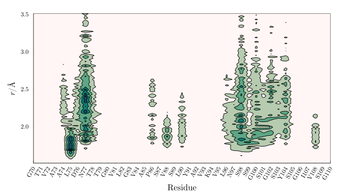
The code above will produce the following plot, which contains, for each residue, the contributions of each residue to the distribution function of glycerol, within 1.5 to 3.5 $\mathrm{\AA}$ of the surface of the protein.

3D density map

In this example we compute three-dimensional representations of the density map of Glycerol in the vicinity of a set of residues of a protein, from the minimum-distance distribution function. For further information about the grid3D function, go to the 3D grid map section of the manual.

import Pkg;
Pkg.activate(".");
using PDBTools
using ComplexMixtures

# PDB file of the system simulated
atoms = readPDB("./system.pdb")

# Load results of a ComplexMixtures run
results = load("./glyc50_results.json")

# Inform which is the solute
protein = select(atoms, "protein")
solute = AtomSelection(protein, nmols=1)

# Compute the 3D density grid and output it to the PDB file
# here we use dmax=3.5 such that the the output file is not too large
grid = grid3D(results, atoms, "./grid.pdb"; dmin=1.5, dmax=3.5)

Here, the MDDF is decomposed at each distance according to the contributions of each solute (the protein) residue. The grid is created such that, at each point in space around the protein, it is possible to identify:

1. Which atom is the closest atom of the solute to that point.

2. Which is the contribution of that atom (or residue) to the distribution function.

Therefore, by filtering the 3D density map at each distance one can visualize over the solute structure which are the regions that mostly interact with the solvent of choice at each distance. Typical images of such a density are:

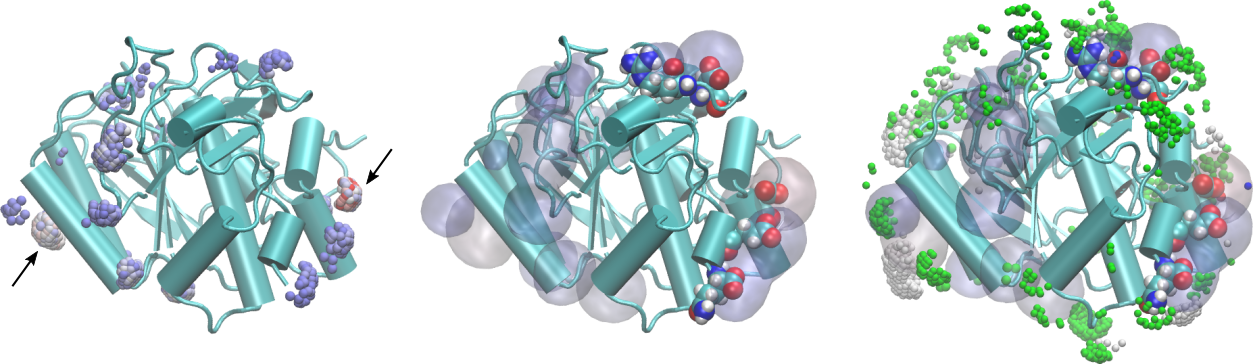
In the figure on the left, the points in space around the protein are selected with the following properties: distance from the protein smaller than 2.0Å and relative contribution to the MDDF at the corresponding distance of at least 10% of the maximum contribution. Thus, we are selecting the regions of the protein corresponding to the most stable hydrogen-bonding interactions. The color of the points is the contribution to the MDDF, from blue to red. Thus, the most reddish-points corresponds to the regions where the most stable hydrogen bonds were formed. We have marked two regions here, on opposite sides of the protein, with arrows.

Clicking on those points we obtain which are the atoms of the protein contributing to the MDDF at that region. In particular, the arrow on the right points to the strongest red region, which corresponds to an Aspartic acid. These residues are shown explicitly under the density (represented as a transparent surface) on the figure in the center.

The figure on the right displays, overlapped with the hydrogen-bonding residues, the most important contributions to the second peak of the distribution, corresponding to distances from the protein between 2.0 and 3.5Å. Notably, the regions involved are different from the ones forming hydrogen bonds, indicating that non-specific interactions with the protein (and not a second solvation shell) are responsible for the second peak.

How to run this example:

Assuming that the input files are available in the script directory, just run the script with:

julia density3D.jl

Alternatively, open Julia and copy/paste or the commands in density3D.jl or use include("./density3D.jl"). These options will allow you to remain on the Julia section with access to the grid data structure that was generated and corresponds to the output grid.pdb file.

This will create the grid.pdb file. Here we provide a previously setup VMD session that contains the data with the visualization choices used to generate the figure above. Load it with:

vmd -e grid.vmd

A short tutorial video showing how to open the input and output PDB files in VMD and produce images of the density is available here: