POPC membrane in water/ethanol

In this example ComplexMixtures.jl is used to study the interactions of a POPC membrane with a mixture of 20%(mol/mol) ethanol in water. At this concentration ethanol destabilizes the membrane.

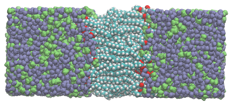
System image: a POPC membrane (center) solvated by a mixture of water (purple) and ethanol (green). The system is composed by 59 POPC, 5000 water, and 1000 ethanol molecules.

Data, packages, and execution

The files required to run this example are:

equilibrated.pdb: The PDB file of the complete system.
traj_POPC.dcd: Trajectory file. This is a 365Mb file, necessary for running from scratch the calculations.

To run the scripts, we suggest the following procedure:

Create a directory, for example example3.
Copy the required data files above to this directory.
Launch julia in that directory: activate the directory environment, and install the required packages. This launching Julia and executing:
```
import Pkg 
Pkg.activate(".")
Pkg.add(["ComplexMixtures", "PDBTools", "Plots", "LaTeXStrings", "EasyFit"])
exit()
```
Copy the code of each script in to a file, and execute with:
```
julia -t auto script.jl
```
Alternativelly (and perhaps preferrably), copy line by line the content of the script into the Julia REPL, to follow each step of the calculation.

MDDF and KB integrals

Here we show the distribution functions and KB integrals associated to the solvation of the membrane by water and ethanol.

Complete example code: click here!

import Pkg;
Pkg.activate(".");

using PDBTools
using ComplexMixtures
using Plots
using LaTeXStrings
using EasyFit: movavg

# The full trajectory file is available at: 
# https://www.dropbox.com/scl/fi/hcenxrdf8g8hfbllyakhy/traj_POPC.dcd?rlkey=h9zivtwgya3ivva1i6q6xmr2p&dl=0
trajectory_file = "./traj_POPC.dcd"

# Load a PDB file of the system
system = readPDB("./equilibrated.pdb")

# Select the atoms corresponding to glycerol and water
popc = select(system, "resname POPC")
water = select(system, "water")
ethanol = select(system, "resname ETOH")

# Set the complete membrane as the solute. We use nmols=1 here such
# that the membrane is considered a single solute in the calculation. 
solute = AtomSelection(popc, nmols=1)

# Compute water-POPC distribution and KB integral 
solvent = AtomSelection(water, natomspermol=3)

# Set the trajectory structure
trajectory = Trajectory(trajectory_file, solute, solvent)

# We want to get reasonably converged KB integrals, which usually
# require large solute domains. Distribution functions converge 
# rapidly (~10Angs or less), on the other side.
options = Options(bulk_range=(15.0, 20.0))

# Compute the mddf and associated properties
mddf_water_POPC = mddf(trajectory, options)

# Save results to file for later use
save(mddf_water_POPC, "./mddf_water_POPC.json")
println("Results saved to ./mddf_water_POPC.json file")

# Compute ethanol-POPC distribution and KB integral 
solvent = AtomSelection(ethanol, natomspermol=9)
traj = Trajectory(trajectory_file, solute, solvent)
mddf_ethanol_POPC = mddf(traj, options)

# Save results for later use
save(mddf_ethanol_POPC, "./mddf_ethanol_POPC.json")
println("Results saved to ./mddf_ethanol_POPC.json file")

#
# Plot the MDDF and KB integrals
#
# Plot defaults
plot_font = "Computer Modern"
default(
    fontfamily=plot_font,
    linewidth=2.5,
    framestyle=:box,
    label=nothing,
    grid=false,
    palette=:tab10
)
scalefontsizes();
scalefontsizes(1.3);

#
# Plots cossolvent-POPC MDDFs in subplot 1
#
plot(layout=(2, 1))
# Water MDDF
plot!(
    mddf_water_POPC.d, # distances
    movavg(mddf_water_POPC.mddf, n=10).x, # water MDDF - smoothed
    label="Water",
    subplot=1
)
# Ethanol MDDF
plot!(
    mddf_ethanol_POPC.d, # distances
    movavg(mddf_ethanol_POPC.mddf, n=10).x, # water MDDF - smoothed
    label="Ethanol",
    subplot=1
)
# Plot settings
plot!(
    xlabel=L"\textrm{Distance / \AA}",
    ylabel="MDDF",
    xlim=(0, 10),
    subplot=1
)

#
# Plot cossolvent-POPC KB integrals in subplot 2
#
# Water KB
plot!(
    mddf_water_POPC.d, # distances
    mddf_water_POPC.kb, # water KB
    label="Water",
    subplot=2
)
# Ethanol KB
plot!(
    mddf_ethanol_POPC.d, # distances
    mddf_ethanol_POPC.kb, # ethanol KB
    label="Ethanol",
    subplot=2
)
# Plot settings
plot!(
    xlabel=L"\textrm{Distance / \AA}",
    ylabel=L"\textrm{KB~/~L~mol^{-1}}",
    xlim=(0, 10),
    subplot=2
)

savefig("popc_water_ethanol_mddf_kb.png")
println("Plot saved to popc_water_ethanol_mddf_kb.png file")

Output

The distribution functions are shown in the first panel of the figure below, and the KB integrals are shown in the second panel.

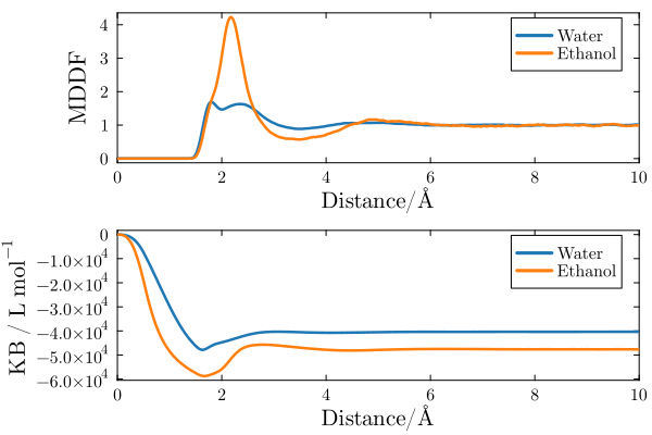
Clearly, both water and ethanol accumulate on the proximity of the membrane. The distribution functions suggest that ethanol displays a greater local density augmentation, reaching concentrations roughly 4 times higher than bulk concentrations. Water has a peak at hydrogen-bonding distances (~1.8$\mathrm{\AA}$) and a secondary peak at 2.5$\mathrm{\AA}$.

Despite the fact that ethanol displays a greater relative density (relative to its own bulk concentration) at short distances, the KB integral of water turns out to be greater (more positive) than that of ethanol. This implies that the membrane is preferentially hydrated.

Ethanol group contributions

The minimum-distance distribution function can be decomposed into the contributions of the ethanol molecule groups.

Complete example code: click here!

import Pkg;
Pkg.activate(".");

using ComplexMixtures
using PDBTools
using Plots
using LaTeXStrings
using EasyFit: movavg

# Some default settings for the plots
plot_font = "Computer Modern"
Plots.default(
    fontfamily=plot_font,
    linewidth=1.5,
    framestyle=:box,
    label=nothing,
    grid=false,
)
scalefontsizes();
scalefontsizes(1.3);

# Read system PDB file
system = readPDB("equilibrated.pdb")
ethanol = select(system, "resname ETOH")

# Load the pre-calculated MDDF of ethanol
mddf_ethanol_POPC = load("mddf_ethanol_POPC.json")

#
# Contributions of the ethanol groups
#
# Define the groups using selections. Set a dict, in which the keys are the group names
# and the values are the selections
groups = (
    "Hydroxyl" => select(ethanol, "name O1 or name HO1"),
    "Aliphatic chain" => select(ethanol, "not name O1 and not name HO1"),
)
# plot the total mddf and the contributions of the groups
x = mddf_ethanol_POPC.d
plot(x, movavg(mddf_ethanol_POPC.mddf, n=10).x, label="Total MDDF")
for (group_name, group_atoms) in groups
    cont = contributions(mddf_ethanol_POPC, SolventGroup(group_atoms))
    y = movavg(cont, n=10).x
    plot!(x, y, label=group_name)
end
# Plot settings
plot!(
    xlim=(1, 8),
    xlabel=L"\textrm{Distance / \AA}",
    ylabel="MDDF"
)
savefig("./mddf_ethanol_groups.png")
println("The plot was saved as mddf_ethanol_groups.png")

In the figure below we show the contributions of the ethanol hydroxyl and aliphatic chain groups to the total MDDF.

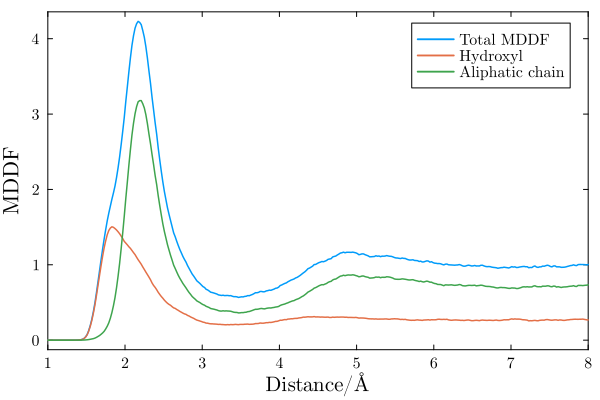
As expected, the MDDF at hydrogen-bonding distances is composed by contributions of the ethanol hydroxyl group, and the non-specific interactions at ~2.5$\mathrm{\AA}$ have a greater contribution of the aliphatic chain of the solvent molecules. It is interesting to explore the chemical complexity of POPC in what concerns these interactions.

Interaction of POPC groups with water

The MDDF can also be decomposed into the contributions of the solute atoms and chemical groups. First, we show the contributions of the POPC chemical groups to the water-POPC distribution.

Complete example code: click here!

import Pkg;
Pkg.activate(".");

using ComplexMixtures
using PDBTools
using Plots
using LaTeXStrings
using EasyFit: movavg

# Some default settings for the plots
plot_font = "Computer Modern"
Plots.default(
    fontfamily=plot_font,
    linewidth=2,
    framestyle=:box,
    label=nothing,
    grid=false,
)
scalefontsizes();
scalefontsizes(1.3);

# Read system PDB file
system = readPDB("equilibrated.pdb")

# Load the pre-calculated MDDF of water
mddf_water_POPC = load("mddf_water_POPC.json")

#
# Here we define the POPC groups, from the atom names. Each group
# is a vector of atom names, and the keys are the group names.
#
groups = (
    "Choline" => ["N", "C12", "H12A", "H12B", "C13", "H13A", "H13B", "H13C", "C14",
        "H14A", "H14B", "H14C", "C15", "H15A", "H15B", "H15C", "C11", "H11A", "H11B"],
    "Phosphate" => ["P", "O13", "O14", "O12"],
    "Glycerol" => ["O11", "C1", "HA", "HB", "C2", "HS", "O21", "C3", "HX", "HY", "O31"],
    "Oleoyl" => ["O22", "C21", "H2R", "H2S", "C22", "C23", "H3R", "H3S", "C24", "H4R", "H4S",
        "C25", "H5R", "H5S", "C26", "H6R", "H6S", "C27", "H7R", "H7S", "C28", "H8R", "H8S",
        "C29", "H91", "C210", "H101", "C211", "H11R", "H11S", "C212", "H12R", "H12S",
        "C213", "H13R", "H13S", "C214", "H14R", "H14S", "C215", "H15R", "H15S",
        "C216", "H16R", "H16S", "C217", "H17R", "H17S", "C218", "H18R", "H18S", "H18T"],
    "Palmitoyl" => ["C31", "O32", "C32", "H2X", "H2Y", "C33", "H3X", "H3Y", "C34", "H4X", "H4Y",
        "C35", "H5X", "H5Y", "C36", "H6X", "H6Y", "C37", "H7X", "H7Y", "C38", "H8X",
        "H8Y", "C39", "H9X", "H9Y", "C310", "H10X", "H10Y", "C311", "H11X", "H11Y",
        "C312", "H12X", "H12Y", "C313", "H13X", "H13Y", "C314", "H14X", "H14Y", "C315",
        "H15X", "H15Y", "C316", "H16X", "H16Y", "H16Z"],
)

#
# plot the total mddf and the contributions of the groups
#
x = mddf_water_POPC.d
plot(
    x,
    movavg(mddf_water_POPC.mddf, n=10).x,
    label="Total water-POPC MDDF"
)
for (group_name, group_atoms) in groups
    cont = contributions(mddf_water_POPC, SoluteGroup(group_atoms))
    y = movavg(cont, n=10).x
    plot!(x, y, label=group_name)
end
# Plot settings
plot!(
    xlim=(1, 5),
    xlabel=L"\textrm{Distance / \AA}",
    ylabel="MDDF"
)
savefig("./mddf_POPC_water_groups.png")
println("The plot was saved as mddf_POPC_water_groups.png")

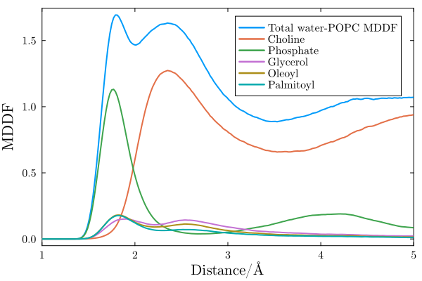
Not surprisingly, water interactions occur majoritarily with the Phosphate and Choline groups of POPC molecules, that is, with the polar head of the lipid. The interactions at hydrogen-bonding distances are dominated by the phosphate group, and non-specific interaction occur mostly with the choline group. Some water molecules penetrate the membrane and interact with the glycerol and aliphatic chains of POPC, but these contributions are clearly secondary.

Interaction of POPC groups with ethanol

The interactions of ethanol molecules with the membrane are more interesting, because ethanol penetrates the membrane. Here we decompose the ethanol-POPC distribution function into the contributions of the POPC chemical groups.

Complete example code: click here!

import Pkg;
Pkg.activate(".");

using ComplexMixtures
using PDBTools
using Plots
using LaTeXStrings
using EasyFit: movavg

# Some default settings for the plots
plot_font = "Computer Modern"
Plots.default(
    fontfamily=plot_font,
    linewidth=2,
    framestyle=:box,
    label=nothing,
    grid=false,
)
scalefontsizes();
scalefontsizes(1.3);

# Read system PDB file
system = readPDB("equilibrated.pdb")

# Load the pre-calculated MDDF of ethanol
mddf_ethanol_POPC = load("mddf_ethanol_POPC.json")

#
# Here we define the POPC groups, from the atom names. Each group
# is a vector of atom names, and the keys are the group names.
#
groups = (
    "Choline" => ["N", "C12", "H12A", "H12B", "C13", "H13A", "H13B", "H13C", "C14",
        "H14A", "H14B", "H14C", "C15", "H15A", "H15B", "H15C", "C11", "H11A", "H11B"],
    "Phosphate" => ["P", "O13", "O14", "O12"],
    "Glycerol" => ["O11", "C1", "HA", "HB", "C2", "HS", "O21", "C3", "HX", "HY", "O31"],
    "Oleoyl" => ["O22", "C21", "H2R", "H2S", "C22", "C23", "H3R", "H3S", "C24", "H4R", "H4S",
        "C25", "H5R", "H5S", "C26", "H6R", "H6S", "C27", "H7R", "H7S", "C28", "H8R", "H8S",
        "C29", "H91", "C210", "H101", "C211", "H11R", "H11S", "C212", "H12R", "H12S",
        "C213", "H13R", "H13S", "C214", "H14R", "H14S", "C215", "H15R", "H15S",
        "C216", "H16R", "H16S", "C217", "H17R", "H17S", "C218", "H18R", "H18S", "H18T"],
    "Palmitoyl" => ["C31", "O32", "C32", "H2X", "H2Y", "C33", "H3X", "H3Y", "C34", "H4X", "H4Y",
        "C35", "H5X", "H5Y", "C36", "H6X", "H6Y", "C37", "H7X", "H7Y", "C38", "H8X",
        "H8Y", "C39", "H9X", "H9Y", "C310", "H10X", "H10Y", "C311", "H11X", "H11Y",
        "C312", "H12X", "H12Y", "C313", "H13X", "H13Y", "C314", "H14X", "H14Y", "C315",
        "H15X", "H15Y", "C316", "H16X", "H16Y", "H16Z"],
)

#
# plot the total mddf and the contributions of the groups
#
x = mddf_ethanol_POPC.d
plot(
    x,
    movavg(mddf_ethanol_POPC.mddf, n=10).x,
    label="Total ethanol-POPC MDDF"
)
for (group_name, group_atoms) in groups
    cont = contributions(mddf_ethanol_POPC, SoluteGroup(group_atoms))
    y = movavg(cont, n=10).x
    plot!(x, y, label=group_name)
end
# Plot settings
plot!(
    xlim=(1.3, 5),
    ylim=(0, 1.8),
    xlabel=L"\textrm{Distance / \AA}",
    ylabel="MDDF"
)
savefig("./mddf_POPC_ethanol_groups.png")
println("The plot was saved as mddf_POPC_ethanol_groups.png")

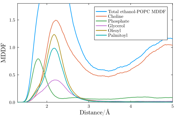
Ethanol molecules interact with the choline and phosphate groups of POPC molecules, as do water molecules. The contributions to the MDDF at hydrogen-bonding distances come essentially from ethanol-phosphate interactions.

However, ethanol molecules interact frequently with the glycerol and aliphatic chains of POPC. Interactions with the Oleoyl chain are slightly stronger than with the Palmitoyl chain. This means that ethanol penetrates the hydrophobic core of the membrane, displaying non-specific interactions with the lipids and with the glycerol group. These interactions are probably associated to the destabilizing role of ethanol in the membrane structure.

Density map on POPC chains

The MDDFs can be decomposed at more granular level, in which each chemical group of the aliphatic chains of the POPC molecules are considered independently. This allows the study of the penetration of the ethanol molecules in the membrane. In the figure below, the carbonyl following the glycerol group of the POPC molecules is represented in the left, and going to the right the aliphatic chain groups are sequentially shown.

Complete example code: click here!

import Pkg;
Pkg.activate(".");

using ComplexMixtures
using PDBTools
using Plots
using LaTeXStrings
using EasyFit: movavg

# Some default settings for the plots
plot_font = "Computer Modern"
Plots.default(
    fontfamily=plot_font,
    linewidth=2,
    framestyle=:box,
    label=nothing,
    grid=false,
)
scalefontsizes();
scalefontsizes(1.3);

# Read system PDB file
system = readPDB("equilibrated.pdb")

# Load the pre-calculated MDDF of ethanol
mddf_ethanol_POPC = load("mddf_ethanol_POPC.json")

# Splitting the oleoyl chain into groups along the the chain. 
# The labels `CH_2` etc stand for `CH₂`, for example, in LaTeX notation, 
# for a nicer plot axis ticks formatting.
oleoyl_groups = (
    "CO" => ["O22", "C21"],
    "CH_2" => ["H2R", "H2S", "C22"],
    "CH_2" => ["C23", "H3R", "H3S"],
    "CH_2" => ["C24", "H4R", "H4S"],
    "CH_2" => ["C25", "H5R", "H5S"],
    "CH_2" => ["C26", "H6R", "H6S"],
    "CH_2" => ["C27", "H7R", "H7S"],
    "CH_2" => ["C28", "H8R", "H8S"],
    "CH" => ["C29", "H91"],
    "CH" => ["C210", "H101"],
    "CH_2" => ["C211", "H11R", "H11S"],
    "CH_2" => ["C212", "H12R", "H12S"],
    "CH_2" => ["C213", "H13R", "H13S"],
    "CH_2" => ["C214", "H14R", "H14S"],
    "CH_2" => ["C215", "H15R", "H15S"],
    "CH_2" => ["C216", "H16R", "H16S"],
    "CH_2" => ["C217", "H17R", "H17S"],
    "CH_3" => ["C218", "H18R", "H18S", "H18T"]
)

# Format tick labels with LaTeX
labels_o = [latexstring("\\textrm{$key}") for (key, val) in oleoyl_groups]

# We first collect the contributions of each group into a vector of vectors:
gcontrib = Vector{Float64}[] # empty vector of vectors
for (group_name, group_atoms) in oleoyl_groups
    group_contributions = contributions(mddf_ethanol_POPC, SoluteGroup(group_atoms))
    push!(gcontrib, movavg(group_contributions; n=10).x)
end

# Convert the vector of vectors into a matrix
gcontrib = stack(gcontrib)

# Find the indices of the MDDF where the distances are between 1.5 and 3.0 Å
idmin = findfirst(d -> d > 1.5, mddf_ethanol_POPC.d)
idmax = findfirst(d -> d > 3.0, mddf_ethanol_POPC.d)

# The plot will have two lines, the first plot will contain the 
# oleoyl groups contributions, and the second plot will contain the
# contributions of the palmitoyl groups.
plot(layout=(2, 1))

# Plot the contributions of the oleoyl groups
contourf!(
    1:length(oleoyl_groups),
    mddf_ethanol_POPC.d[idmin:idmax],
    gcontrib[idmin:idmax, :],
    color=cgrad(:tempo), linewidth=1, linecolor=:black,
    colorbar=:none, levels=10,
    ylabel=L"r/\AA", xrotation=60,
    xticks=(1:length(oleoyl_groups), labels_o),
    subplot=1,
)
annotate!(14, 2.7, text("Oleoyl", :left, 12, plot_font), subplot=1)

#
# Repeat procedure for the palmitoyl groups
#
palmitoyl_groups = (
    "CO" => ["C31", "O32"],
    "CH_2" => ["C32", "H2X", "H2Y"],
    "CH_2" => ["C33", "H3X", "H3Y"],
    "CH_2" => ["C34", "H4X", "H4Y"],
    "CH_2" => ["C35", "H5X", "H5Y"],
    "CH_2" => ["C36", "H6X", "H6Y"],
    "CH_2" => ["C37", "H7X", "H7Y"],
    "CH_2" => ["C38", "H8X", "H8Y"],
    "CH_2" => ["C39", "H9X", "H9Y"],
    "CH_2" => ["C310", "H10X", "H10Y"],
    "CH_2" => ["C311", "H11X", "H11Y"],
    "CH_2" => ["C312", "H12X", "H12Y"],
    "CH_2" => ["C313", "H13X", "H13Y"],
    "CH_2" => ["C314", "H14X", "H14Y"],
    "CH_2" => ["C315", "H15X", "H15Y"],
    "CH_3" => ["C316", "H16X", "H16Y", "H16Z"],
)

# Format tick labels with LaTeX
labels_p = [latexstring("\\textrm{$key}") for (key, val) in palmitoyl_groups]

# We first collect the contributions of each group into a # vector of vectors:
gcontrib = Vector{Float64}[] # empty vector of vectors
for (group_name, group_atoms) in palmitoyl_groups
    group_contributions = contributions(mddf_ethanol_POPC, SoluteGroup(group_atoms))
    push!(gcontrib, movavg(group_contributions; n=10).x)
end

# Convert the vector of vectors into a matrix
gcontrib = stack(gcontrib)

# Plot the contributions of the palmitoyl groups
contourf!(
    1:length(palmitoyl_groups),
    mddf_ethanol_POPC.d[idmin:idmax],
    gcontrib[idmin:idmax, :],
    color=cgrad(:tempo), linewidth=1, linecolor=:black,
    colorbar=:none, levels=10,
    xlabel="Group",
    ylabel=L"r/\AA", xrotation=60,
    xticks=(1:length(labels_p), labels_p),
    bottom_margin=0.5Plots.Measures.cm,
    subplot=2,
)
annotate!(12, 2.7, text("Palmitoyl", :left, 12, plot_font), subplot=2)

savefig("POPC_ethanol_chains.png")
println("The plot was saved as POPC_ethanol_chains.png")

#
# Now, plot a similar map for the water interactions with the POPC chain
#
mddf_water_POPC = load("mddf_water_POPC.json")
plot(layout=(2, 1))

# Plot the contributions of the oleoyl groups
# We first collect the contributions of each group into a vector of vectors:
gcontrib = Vector{Float64}[] # empty vector of vectors
for (group_name, group_atoms) in oleoyl_groups
    group_contributions = contributions(mddf_water_POPC, SoluteGroup(group_atoms))
    push!(gcontrib, movavg(group_contributions; n=10).x)
end
# Convert the vector of vectors into a matrix
gcontrib = stack(gcontrib)
# Plot matrix as density map
contourf!(
    1:length(oleoyl_groups),
    mddf_water_POPC.d[idmin:idmax],
    gcontrib[idmin:idmax, :],
    color=cgrad(:tempo), linewidth=1, linecolor=:black,
    colorbar=:none, levels=10,
    ylabel=L"r/\AA", xrotation=60,
    xticks=(1:length(oleoyl_groups), labels_o), subplot=1,
)
annotate!(14, 2.7, text("Oleoyl", :left, 12, plot_font), subplot=1)

# Plot the contributions of the palmitoyl groups
# We first collect the contributions of each group into a vector of vectors:
gcontrib = Vector{Float64}[] # empty vector of vectors
for (group_name, group_atoms) in palmitoyl_groups
    group_contributions = contributions(mddf_water_POPC, SoluteGroup(group_atoms))
    push!(gcontrib, movavg(group_contributions; n=10).x)
end
# Convert the vector of vectors into a matrix
gcontrib = stack(gcontrib)
# Plot matrix as density map
contourf!(
    1:length(palmitoyl_groups),
    mddf_water_POPC.d[idmin:idmax],
    gcontrib[idmin:idmax, :],
    color=cgrad(:tempo), linewidth=1, linecolor=:black,
    colorbar=:none, levels=10,
    xlabel="Group",
    ylabel=L"r/\AA", xrotation=60,
    xticks=(1:length(palmitoyl_groups), labels_o),
    subplot=2,
    bottom_margin=0.5Plots.Measures.cm,
)
annotate!(12, 2.7, text("Palmitoyl", :left, 12, plot_font), subplot=2)

savefig("POPC_water_chains.png")
println("The plot was saved as POPC_water_chains.png")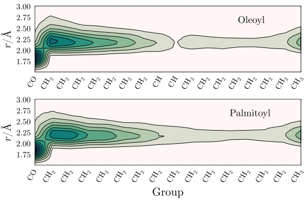

Ethanol displays an important density augmentation at the vicinity of the carbonyl that follows the glycerol group, and accumulates on the proximity of the aliphatic chain. The density of ethanol decreases as one advances into the aliphatic chain, displaying a minimum around the insaturation in the Oleoyl chain. The terminal methyl group of both chains display a greater solvation by ethanol, suggesting the twisting of the aliphatic chain expose these terminal groups to membrane depth where ethanol is already abundant.

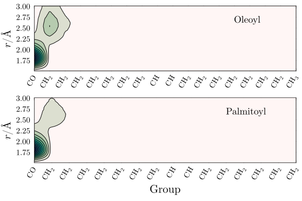
The equivalent maps for water are strikingly different, and show that water is excluded from the interior of the membrane:

References

Membrane built with the VMD membrane plugin.

Water and ethanol layers added with Packmol.

The simulations were performed with NAMD, with CHARMM36 parameters.

Density of the ethanol-water mixture from: https://wissen.science-and-fun.de/chemistry/chemistry/density-tables/ethanol-water-mixtures/