PACKMOL

Initial configurations for Molecular Dynamics Simulations by packing optimization

Institute of Chemistry and Institute of Mathematics
University of Campinas
Institute of Mathematics and Statistics
University of São Paulo

Packmol:

Download
Input Examples
User guide
Utilities
External links
Applications

Reference:

Citation
Features
Version history

Contact:

E-mail
Regular mail

User guide

Important: always download the latest version of Packmol in order that all features are available.

Contents
1. What do you need?
2. How to compile Packmol.
3. Running Packmol.
4. Basic input structure.
5. More types of molecules.
6. Atom selections.
7. Types of constraints.
8. Periodic boundary conditions.
9. Different radii for different atoms.
10. Solvating a large molecule automatically.
11. Controlling residue numbering in PDB files.
12. Building very large systems: using restart files.
13. Convergence problems: what to try.
14. Additional input options and keywords.
15. Some tutorials available online.

What do you need?

You need coordinate files for each type of molecule you want your simulation to have. For example, if you are going to simulate a solution of water and ions, you will need a coordinate file for one water molecule, and independent coordinates files for each of the ions. This coordinate files may be in the PDB, TINKER, MOLDEN or MOLDY format. The simplest and best molecular structure builder we have used is this one.

Of course, you also need the Packmol package, which you can get from

  http://m3g.iqm.unicamp.br/packmol

by clicking on the Download link. You can download the file packmol-20.14.2.tar.gz which contains the whole source code of Packmol. The 20.13.0 is the version number, which might change relative to this example.

Windows users: We suggest trying to use the Julia-based distribution available at [Packmol.jl], which works on all platforms and doesn't need compilation.

If you plan to use MOLDY as your MD package, read THIS.

How to compile Packmol

Once you have downloaded the packmol-20.13.0.tar.gz file from the home-page, you need to expand the files and compile the package. This is done by:

Expanding the files:

  tar -xvzf packmol-20.13.0.tar.gz

This will create a directory called packmol inside which you can find the source code. You can build the executable by:

  cd packmol
  make

That's it, if no error was reported the packmol executable was built. Note that 20.13.0 is the version number, which may differ relative to this example.

-----

If you have problems, let the configure script find a suitable compiler for you:

chmod +x ./configure (this makes the script executable)

./configure (this executes the script)

If the script was not able to find a suitable compiler, then you can manually set the compiler by:

./configure /path/to/your/compiler/yourcompiler

Then, run the "make" command again:

make

If no error was detected, an executable called packmol is now ready.

Running Packmol

Once you have compiled and built your input file, run Packmol with

packmol < packmol.inp Where packmol.inp is the input file (you can obtain example files by clicking at the 'Input examples' link on the left).

A successful packing will end with something like ------------------------------ Success! Final objective function value: .22503E-01 Maximum violation of target distance: 0.000000 Maximum violation of the constraints: .78985E-02 ------------------------------ Where the maximum violation of the target distance indicates the difference between the minimum distance between atoms required by the user and that of the solution. It will not be greater than 10^-2 The maximum violation of the constrains must not be greater than 10^-2.

A good idea is to check if your constraints are correct by using the "check" keyword in the input file. With this option a rough initial approximation will be built but no actual packing will be performed. You can look at the output to see if the molecules are within the desired regions (but do not expect a good structure at this point!). Just add the word "check" to any line of your input file (available since 28 Feb 2008).

Common issues:

- If you get "Command not found" when running Packmol, use
./packmol < packmol.inp
(with a "./" before "packmol") or add the directory where the packmol executable is located to your path.

- If you run packmol and get the message "Killed", this is because the package is trying to allocate more memory than available for static storage. Open the "sizes.i" file and decrease the "maxatom" parameter to the number of atoms of your system, compile the package again, and try again.

Basic input structure

The minimal input file must contain the distance tolerance required (for systems at room temperature and pressure and coordinates in Angstroms, 2.0 Å is a good value [note]). This is specified with

tolerance 2.0

The file must contain also the name of the output file to be created, specified with

output test.pdb

and the file type (pdb, tinker, xyz or moldy, pdb is the default value),

filetype pdb

At least one type of molecule must be present. This is set by the structure ... end structure section, for example, if water.pdb is the file containing the coordinates of a single water molecule, you could add to your input file something like

structure water.pdb   number 2000   inside cube 0. 0. 0. 40. end structure

This section specifies that 2000 molecules of the water.pdb type, will be placed inside a cube with minimum coordinates $(x,y,z) = (0,0,0)$ and maximum coordinates $(40,40,40)$. Therefore, this minimum input file must be:

tolerance 2.0 output test.pdb filetype pdb structure water.pdb   number 2000   inside cube 0. 0. 0. 40. end structure

Running Packmol with this input file will fill a cube of side 40.0 Å with 2000 water molecules. Every pair of atoms of different molecules will be separated by, at least, 2.0 Å and the molecules will be randomly distributed inside de cube.

More types of molecules

You can add more types of molecules to the same region, or to different regions of the space, simply adding other structure ... end structure section to the input file.

Atom selections

The coordinate file of a single molecule contains, for example, 10 atoms. You can restrain a part of the molecule to be in a specified region of the space. This is useful for building vesicles where the hydrophilic part of the surfactants must be pointing to the aqueous environment, for example. For the 10 atoms molecule, this is done by using the keyword atoms, as in

structure molecule.pdb   inside cube 0. 0. 0. 20.   atoms 9 10     inside box 0. 0. 15. 20. 20. 20.   end atoms end structure

In this case, all the atoms of the molecule will be put inside the defined cube, but atoms 9 and 10 will be restrained to be inside the box.

Types of constraints

There are several types of constraints that can be applied both to whole molecules or to parts of the molecule. These constraints define the region of the space in which the molecules must be at the solution. Very ordered systems can be built in such a way. The constraints are:

1.	`fixed`
	Usage: `fixed` x y z a b g This options holds the molecule fixed in the position specified by the parameters. x, y, z, a, b, g, which are six real numbers. The first three determine the translation of the molecule relative to its position in the coordinate file. The former three parameters are rotation angles (in radians). For this option it is required that only one molecule is set. It may be accompanied by the keyword `center`. If this keyword is present the first three numbers are the position of the baricenter (not really the center of mass, because we suppose that all atoms have the same mass). Therefore this keyword must be used in the following context: `structure molecule.pdb number 1 center fixed 0. 0. 0. 0. 0. 0. end structure` In this example, the molecule will be fixed with its center the origin and no rotation.
2.	`inside cube`
	Usage: `inside cube` x_min y_min z_min d x_min , y_min , z_min and d are four real numbers. The coordinates (x,y,z) of the atoms restrained by this option will satisfy, at the solution: x_min < x < x_min + d y_min < y < y_min + d z_min < z < z_min + d
3.	`outside cube`
	Usage: `outside cube` x_min y_min z_min d x_min , y_min , z_min and d are four real numbers. The coordinates (x,y,z) of the atoms restrained by this option will satisfy, at the solution: x < x_min or x > x_min + d y < y_min or y > y_min + d z < z_min or z > z_min + d
4.	`inside box`
	Usage: `inside box` x_min y_min z_min x_max y_max z_max x_min , y_min , z_min , x_max , y_max and z_max are six real numbers. The coordinates (x,y,z) of the atoms restrained by this option will satisfy, at the solution: x_min < x < x_max y_min < y < y_max z_min < z < z_max
5.	`outside box`
	Usage: `outside box` x_min y_min z_min x_max y_max z_max x_min , y_min , z_min , x_max , y_max and z_max are six real numbers. The coordinates (x,y,z) of the atoms restrained by this option will satisfy, at the solution: x < x_min or x > x_max y < y_min or y > y_max z < z_min or z > z_max
6.	`inside (or outside) sphere`
	Spheres are defined by equations of the general form $$ (x - a)^2 + (y - b)^2 + (z - c)^2 - d^2 = 0 $$ and, therefore, you must provide four real parameters a, b, c and d in order to define it. The input syntax is, for example, `inside sphere 2.30 3.40 4.50 8.0` and therefore the coordinates of the atoms will satisfy the equation $$ (x - 2.30)^2 + (y - 3.40)^2 + (z - 4.50)^2 - 8.0^2 \leq 0.0 $$ Other input alternative would be: `outside sphere 2.30 3.40 4.50 8.0` The `outside` parameter is similar to the `inside` parameter, but the equation above uses $\geq$ instead of $\leq$ and, therefore, the atoms will be placed outside the defined sphere.
7.	`inside (or outside) ellipsoid`
	Ellipsoids are defined by the general equation $$ \frac{(x-a_1)^2}{a_2^2} + \frac{(y-b_1)^2}{b_2^2} + \frac{(z-c_1)^2}{c_2^2} - d² = 0 $$ The parameters must be given as in the sphere example, but now they are 7, and must be entered in the following order: `inside ellipsoid` a₁ b₁ c₁ a₂ b₂ c₂ d The coordinates (a₁,b₁,c₁) will define the center of the ellipsoid, the coordinates (a₂,b₂,c₂) will define the relative size of the axes and d will define the volume of the ellipsoid. Of course, the commands `outside ellipsoid` a₁ b₁ c₁ a₂ b₂ c₂ d can also be used in the same manner as the parameters for spheres. Note that the case a₂ = b₂ = c₂ = 1.0 provides the exactly the same as the sphere parameter. The parameters for the ellipsoid are not normalized. Therefore, if a₂, b₂ and c₂ are large, the ellipsoid will be large, even for a small d.
8.	`above (or below) plane`
	The planes are defined by the general equation $$ ax + by + cz - d = 0 $$ And it is possible to restrict atoms to be above or below the plane. The syntax is `above plane 2.5 3.2 1.2 6.2 below plane 2.5 3.2 1.2 6.2` where the `above` keyword will make the atoms satisfy the condition $$ 2.5x + 3.2y + 1.2z - 6.2 \geq 0 $$ and the `below` keyword will make the atoms satisfy $$ 2.5x + 3.2y + 1.2z - 6.2 \leq 0 $$ *Note: the `above` notation was introduced in version 20.1.1 (Sept. 5, 2020)
9.	`inside (or outside) cylinder`
	In order to define a cylinder, it is necessary first to define a line oriented in space. This line is defined in `Packmol` by the parametric equation $$ p = (a_1, b_1, c_1) + t \times (a_2, b_2, c_2) $$ where $t$ is the independent parameter. The vector $(a_2, b_2, c_2)$ defines the direction of the line. The cylinder is therefore defined by the distance to this line, $d$, and a length $l$. Therefore, the usage must be: inside cylinder a₁ b₁ c₁ a₂ b₂ c₂ d l outside cylinder a₁ b₁ c₁ a₂ b₂ c₂ d l Here, the first three parameters define the point where the cylinder starts, and l defines the length of the cylinder. d defines de radius of the cylinder. The simpler example is a cylinder oriented in the x axis and starting at the origin, such as `inside cylinder 0. 0. 0. 1. 0. 0. 10. 20.` This cylinder is specified by the points that have a distance of 10. to the x axis (the cylinder has a radius of 10.). Furthermore, it starts at the origin, therefore no atom restricted by this cylinder will have an x coordinate less than 0. Furthermore, it has a length of 20. and, as such, no atom will have an x coordinate greater than 20. The orientation of the cylinder, parallel to the x axis is defined by the director vector (1,0,0), the fourth, fifth and sixth parameters. Cylinders can be oriented in space in anyway.
10.	`Constrain rotations`
	It is possible to constrain rotations of all molecules of each type, so that they have some average orientation in space. The keywords to be used are, within a structure...end structure section: `constrain_rotation x 180. 20. constrain_rotation y 180. 20. constrain_rotation z 180. 20.` Each of these keywords restricts the possible rotation angles around each axis to be within 180±20 degrees (or any other value). For a technical reason the rotation around the `z` axis will, alone, be identical to the rotation around the `y` axis (we hope to fix this some day). Constraining the three rotations will constrain completely the rotations. Note that to have your molecules oriented parallel to an axis, you need to constrain the rotations relative to the other two. For example, to constrain the rotation of your molecule along the `z` axis, use something like: `constrain_rotation x 0. 20. constrain_rotation y 0. 20.` Note that these rotations are defined relative to the molecule in the orientation which was provided by the user, in the input PDB file. Therefore, it is a good idea to orient the molecule in a reasonable way in order to understand the rotations. For example, if the molecule is elongated in one direction, a good idea is to provide the molecule with the larger dimension oriented along the `z` axis.
11.	`over (or below) xygauss` (gaussian surface)
	Gaussian surfaces are defined by the equation $$ h \times exp\left[−\frac{(x-a_1)^2}{2a_2^2}−\frac{(y-b_1)^2}{(2b_2^2)}\right]-(z-c)=0 $$ Parameters $(a_1, b_1)$ define center of the gaussian, while $c$ specifies the height in the $z$ dimension. $a_2$ and $b_2$ set the width of the gaussian in $x$ and $y$, respectively, while $h$ specifies its height. It is possible to restrict atoms to be over or below the gaussian plane. The gaussian surface as implemented is restricted to be over the $xy$ plane. The syntax is `over xygauss a₁ b₁ a₂ b₂ c h` `below xygauss a₁ b₁ a₂ b₂ c h` For example, using `over xygauss 21.0 5.0 10.0 20.0 -23.0 15.0` the atoms satisfy the condition $$ 15.0 \times exp\left[−\frac{(x-21.0)^2}{2(10.0)^2}−\frac{(y-5.0)^2}{2(20.0)^2}\right]-(z+23.0) \geq 0.0 $$

Periodic Boundary Conditions

Periodic Boundary Conditions for cubic and rectangular boxes are often requested by users. We aim to implement that in the future. At the same time, there is a simple workaround we suggest: If your system will be simulated in a, for example, 100. Angs box, define your cubic constraints such that the packing is done in a 98. Angs box. That way, when the actual simulation box with PBC is built, images will be 2. Angs apart from each other, as illustrated in the figure below. There will be an empty space at the boundary, but that will readily disappear with energy minimization and equilibration.

Different radii for different atoms

It is possible (from version 15.133 on) to attribute different radii to different atoms during the packing procedure. The default behavior is that all atoms will be distant to each other at the final structure at least the distance defined by the tolerance parameter. In this case it is possible to think that the radius of every atom is half the distance tolerance. A tolerance of 2.0 Angs is usually fine for simulation of molecular systems using all-atom models.

Most times, therefore, you won't need this option. This was requested by users that want to pack multiscale models, in which all-atom and coarse-grained representations are combined in the same system.

It is easy to define different radii to different molecules, or to atoms within a molecule. Just add the "radius" keyword within the structure ... end structure section of a molecule type, or within atoms ... end atoms section of an atom selection.

For example, in this case:


tolerance 2.0

structure water.pdb

  number 500

  inside box 0. 0. 0. 30. 30. 30.

  radius 1.5

end structure

the radius of the atoms of the water molecules will be 1.5. Note that this implies a distance tolerance of 3.0 within water molecules.

In this case, on the other side:


tolerance 2.0

structure water.pdb

  number 500

  inside box 0. 0. 0. 30. 30. 30.

  atoms 1 2

    radius 1.5

  end atoms

end structure

only atoms 1 and 2 of the water molecule (as listed in the water.pdb file) will have a radius of 1.5, while atom 3 will have a radius of 1.0, as defined by the tolerance of 2.0

Always remember that the distance tolerance is the sum of the radii of each pair of atoms, and that the greatest the radii the harder the packing. Also, keep in mind that your minimization and equilibration will take care of the actual atom radii, and Packmol is designed only to give a first coordinate file.

Finally, currently the restrictions are set to be fulfilled by the center of the atoms. Therefore, if you are using large radii, you might want to adjust the sizes of the boxes, spheres, etc., so that the whole atoms are within the desired regions. For standard all-atom simulations this is not usually an issue because the radii are small.

Solvating large molecules automatically

The Packmol distribution includes the solvate.tcl script, which is used to solvate large molecules, usually proteins, with water and ions (Na⁺ and Cl^-). Given the PDB file of the biomolecule, just run the script with:


solvate.tcl PROTEIN.pdb

And the script will create a input file for packmol called packmol_input.inp. With this file, run Packmol with

packmol < packmol_input.inp

And your large molecule will be solvated by a shell of 15. Angs. of water, and ions to keep the system neutral and a physiological NaCl concentration of 0.16M. The script usually makes reasonable choices for every parameter (number of water molecules, number of ions, etc.), but these may be controlled manually with additional options, as described below:


solvate.tcl structure.pdb -shell 15. -charge +5 -density 1.0 -i pack.inp
-o solvated.pdb

Where: structure.pdb is the pdb file to be solvated (usually a protein)

"15." is the size of the solvation shell. This is an optional parameter. If not set, 15. will be used.

+5 is the total charge of the system, to be neutralized. This is also and optional parameter, if not used, the package considers histidine residues as neutral, Arg and Lys as +1 and Glu and Asp as -1. The Na+ and Cl- concentrations are set the closest possible to 0.16M, approximately the physiological concentration. Alternatively, use the -noions to not add any ions, just water.

1.0 is the desired density. Optional. If not set, the density will be set to 1.0 g/ml.

solvated.pdb: is the (optional) name for the solvated system output file. If this argument is not provided, it will be the default solvated.pdb file.

pack.inp: is the (optional) name for the packmol input file that will be generated. If not provided, packmol_input.inp will be used.

All these options are output when running the "solvate.tcl" script without any parameter. The script also outputs the size of the box and the suggested periodic boundary condition dimensions to be used.

Controlling residue numbering in PDB files.

Since Packmol will create one or more copies of your molecules in a new PDB file, there are some options on how residue numbers are set to these new molecules. There are four options, which are set with the resnumbers keyword. This keyword may assume three values, 0, 1, 2 or 3, and must be inserted within the structure ... end structure section of each type of molecule. The options are:

resnumbers 0

In this case the residue numbers of all residues will correspond to the molecule of each type, independently of the residue numbering of the original pdb file. This means that if you pack 10 water molecules and 10 ethanol molecules, the water molecules will be numbered 1 to 10, and the ethanol molecules will be numbered 1 to 10.

resnumbers 1

In this case, the residue numbers of the original pdb files are kept unmodified. This means that if you pack 10 proteins of 5 residues, the residue numbers will be preserved and, therefore, they will be repeated for equivalent residues in each molecule of the same protein.

resnumbers 2

In this case, the residue numbers of all residues for this structure will be numbered sequentially according to the number of residues that are printed previously in the same file. This means that if you pack 10 proteins of 5 residues, there will be residue numbers ranging from 1 to 50.

resnumbers 3

In this case, the numbering of the residues will correspond to the sequential numbering of all residues in the file. That is, if you pack a protein with 150 residues followed by 10 water molecules, and use this option for the water molecules, the water molecules will be numbered from 151 to 161. Note: If you use this option for a protein, the whole protein will have its residue numbers overwritten by the same number, corresponding to the residue that would follow in the complete structure.

For example, this keyword may be used as in:

structure peptide.pdb  
  number 10               
  resnumbers 1            
  inside box 0. 0. 0. 20. 20. 20.
end structure

Default: The default behavior is to use 0 for structures with only one residue and 1 for structures with more than one residue.

Chain identifier:
It is also possible to modify the "chain" identifiers of PDB files. By default, each type of molecule is set to a "chain". On the other side, using the

changechains

whithin the structure...end structure section of a type of molecule, the chains will alternate between two values ("A" and "B" for example). This might be useful if the molecules are peptides, and topology builders sometimes think that the peptides of the same chain must be joint by covalent bonds. This is avoided by alternating the chain from molecule to molecule.

Additionally each structure can have a specific chain identifier, set by the user with the option:

chain D

where "D" is the desired identifier (Do not use "#").

Building very large systems: using restart files

From version 16.143 on, it is possible to build the system from multiple and independent executions of Packmol by the use of restart files. In order to write a restart file, the following keyword must be used: restart_to restart.pack where restart.pack is the name of the restart file to be created. It is possible to write restart files for the whole system, if the keyword is put outside structure...end structure sections, or to write a restart file for a specific part of the system, using, for instance:

structure water.pdb
  number 1000
  inside cube 0. 0. 0. 40.
  restart_to water1.pack
end structure

This will generate a restart file for the water molecules only.

These restart files can be used to start a new execution of Packmol with more molecules. The restart_from keyword must then be used. For example:

structure water.pdb
  number 1000
  inside cube 0. 0. 0. 40.
  restart_from water1.pack
end structure

The new input file might contain other molecules, as a regular Packmol input file, and these water molecules will be packed together with the new molecules, but starting from the previous runs. This can be used, for example, to build solvated bilayers by parts. For instance, the bilayers could be built and, later, different solvents can be added to the bilayer, without having to restart the whole system construction from scratch every time. This could also be used to add some molecule to the bilayer.

Tip: the restart file can be used to restart the position of a smaller number of molecules of the same type. For instance, if a new molecule is introduced inside a previous set of molecules (a lipid bilayer, for instance), you can tell Packmol to pack less molecules of the original set, in order to provide space for the new structure, while using the original restart file of more molecules. That is, a restart_from water1.pack similar to the ones of the example above could be used to restart the positions of 800 molecules.

Convergence problems: what to try

Sometimes Packmol is not able to find an adequate packing solution. Here are some tips to try to overcome these difficulties:

• Look at the best solution obtained, many times it is good enough to be used.

• Simulate the same problem with only a few molecules of each type. For example, instead of using 20 thousand water molecules, put 300, and see if they are in the correct regions.

• If you have large molecules, try running the program twice, one to pack these molecules, and then use the solution as fixed molecule for the next packing, in which solvation is included. This may be particularly useful for building solvated membranes. Build the membrane first and then use it as a fixed molecule for a solvation run.

• You can change some options of the packing procedure to try improve the optimization:

1.	`discale [real]` This option controls the distance tolerance actually used in the local optimization method. It was found that using larger distances helps sometimes. Try setting `discale` to 1.5, for example.
2.	`maxit [integer]` This is the maximum number of iterations of the local optimizer (GENCAN) per loop. The default value is currently 20, changing it may improve (or worse) the convergence.
3.	`movebadrandom` One of the convergence heuristics of Packmol consists in moving molecules that are badly placed. If this option is set, the molecules will be placed in new random position in the box. If not (default), the molecules are moved to positions nearby molecules that are well packed. Using this option can help when the restraints are complex, but will probably be bad if there are large structures, because the new random position might overlap with those.
4.	`movefrac` and `maxmove` In the heuristic that moves the worst molecules, `movefrac` defines which is the fraction of molecules that are going to be moved, for each type of molecule. For very large systems, it is isually a good idea to define a small value of `movefrac`, because otherwise the randomization of the system is too great. The default value is 0.05. At the same time, `maxmove` defines a maximum absolute number of molecules to be displaced for each type of molecule. it must be set within a `structure ... end structure` section, and defaults to the number of molecules of each type.

Additional input options and keywords

There are some input options which are probably not of interest of the general user, but may be useful in specific contexts. These keywords may be added in the input file in any position.

Write a CHARMM CRD file as output:
Usage: writecrd output.crd
The segment identifier for each type of molecule can be set by adding, within the structure ... end structure section of each type, the following keyword:
segid NAME.

Add the TER flag betwen every molecule (AMBER uses this):
Usage: add_amber_ter
and
Usage: amber_ter_preserve
(this option will preserve TER flags within input structures, fixed or not from v20.14.0 on).

Add box side information to output PDB File (GROMACS uses this):
Usage: add_box_sides 1.0
Where the "1.0" is an optional real number that will be added to the length of each side, if the actual sides of your simulation box will not be exactly the same as the maximum and minimum coordinates of the molecules of the system (usually, if you are using periodic boundary conditions, you may want to add "1.0" to avoid clashes at the boundary).

Display, or not, connectivity of molecules in output PDB files:
Usage: connect yes/no
By default, if the input PDB file of a molecule has CONECT fields, the output PDB File of packmol will contain also CONECT fields with the appropriate connectivity of the corresponding molecules. If you do not want this, add connect no to the structure section of this molecule, and the output of the connectivity will be suppressed.

Increase maximum system dimensions:
Usage: sidemax [real] (ex: sidemax 2000.d0)
"sidemax" is used to build an initial approximation of the molecular distribution. Increase "sidemax" if your system is very large, or your system may look cut out by this maximum dimension. All system coordinates must fit within -sidemax and +sidemax, and using a sidemax that approximately fits your system may accelerate a little bit the packing calculation. The default value is 1000.d0.

Change random number generator seed:
Usage: seed [integer] (ex: seed 191917)
Use seed -1 to generate a seed automatically from the computer time.

Use a truly random initial point for the minimization (the default option is to generate a roughly homogeneous-density initial approximation):
Usage: randominitialpoint

Avoid, or not, overlap with fixed molecules at initial point (avoiding this overlaps is generally recommended, but sometimes generates gaps that are too large):
Usage: avoid_overlap yes/no

Change the maximum number of Gencan iterations per loop:
Usage: maxit [integer]

Change the maximum number of optimization loops (if this option is used inside the structure section, it affects the number of optimization loops only of that specific structure):
Usage: nloop [integer]

Change the precision required for the solution: how close the solution must be to the desired distances to be considered correct.
Usage: precision [real] (Default: 0.01)

Change the frequency of output file writing:
Usage: writeout [integer]

Write the current point to output file even if it is worse than the the best point so far (used for checking purposes only):
Usage: writebad

Change the optimization subroutine printing output:
Usage: iprint1 [integer] and/or iprint2 [integer]
where the integer must be 0, 1, 2 or 3.

Change the number of bins of the linked-cell method (technical):
Usage: fbins [real]
The default value is the square root of three.

Compare analytical and finite-difference gradients: This is only for testing purposes. Writes chkgrad.log file containing the comparison.
Usage: chkgrad

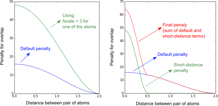
Options tho change the shape of the minimum-distance penalty function:

Usage: fscale [real]
This option must be used within structure ... end structure or atoms ... end atoms sections, to change the weight of the penalty function, as illustrated in the images below. The fscale defines how greater the penalty is relative to the default penalty.

Usage: use_short_tol
Usage: short_tol_dist [real]
Usage: short_tol_scale [real]
These options define a new penalty tolerance for short distances, to increase the repulsion between atoms when they are too close to each other. The "use" parameter turns on this feature, using default parameters (dist=tolerance/2; scale=3). The "dist" parameter defines from which distance the penalty is applied, and the "scale" parameter how greater this penalty is relative to the default penalty. They affect the penalty of all atoms. Remember that the "tolerance" is twice the size of the "radius" of each atom. The figure below, on the right, illustrates for example the build up of the penalty function using short_tol_dist=0.5; short_tol_scale=3, with the default overall tolerance of 2.0 set.

Usage: short_radius [real]
Usage: short_radius_scale [real]
These parameters define a new penalty for short distances, but for specific atoms. These options must be used within structure ... end structure or atoms ... end atoms sections. Note that, in this case, the radius is defined (the actual tolerance is the sum of the radii of each pair of atoms; for atoms without an explicit radius definition, the radius is one half of the overall set tolerance parameter).

Third party tutorials:

Here are some tutorials developed by third-parties which might be useful:

Install and Run Packmol on Window 10
by: Vinay Thakur

Packmol Software Using in Windows 10
by: LAMMPS Tube

Windows: Tutorial - Using Packmol to generate solvation shell around molecules.
by: Filipe Camargo Dalmatti Alves Lima

PACKMOL tutorial- Solvation of proteins in non-standard solvents
by: Mohamed Shehata

Preparation of initial configuration of polymers for MD simulation
by: Jeremy Wong