Solvent Accessible Surface Area (SASA)

These functions are used to compute the solvent accessible surface area (SASA) of structures or parts of a structure. They provide a very fast implementation of the Shake-Rupley method, using a Fibonacci lattice to construct the grid points.

sasa_particles(atoms; probe_radius, n_dots)

julia> using PDBTools

julia> prot = select(read_pdb(PDBTools.TESTPDB), "protein");

julia> at_sasa = sasa_particles(prot);

julia> sasa(at_sasa) # total sasa of prot
5389.0146f0

julia> sasa(at_sasa, "backbone") # backbone sasa in prot
988.7648f0

julia> sasa(at_sasa, "not backbone") # other atoms
4400.246f0

julia> sasa(at_sasa, "resname ARG GLU") # some residue types
543.29846f0

sasa_particles(StandardAtomicRadii, atoms; kargs...)

sasa_particles(CreamerUnitedAtomRadii, atoms; kargs...)

sasa_particles(RichardsUnitedAtomRadii, atoms; radii_set=:set2, kargs...)

sasa(s::SASA)
sasa(s::SASA{<:AbstractVector{<:PDBTools.Atom}})
sasa(atoms::SASA{<:AbstractVector{PDBTools.Atom}}, selection::Union{Function,String})

julia> using PDBTools

julia> prot = select(read_pdb(PDBTools.TESTPDB), "protein");

julia> at_sasa = sasa_particles(prot);

julia> sasa(at_sasa) # total sasa of prot
5389.0146f0

julia> sasa(at_sasa, "backbone") # selection string
988.7648f0

julia> sasa(at_sasa, at -> name(at) == "CA") # selection function
44.078426f0

julia> sasa(at_sasa[1]) # single atom SASA
5.467941f0

Complete structure SASA

A typical run of these functions consists in providing the structure of a protein to the first function, sasa_particles, to obtain a SASA object, which contains the accessible area per atom:

using PDBTools
prot = read_pdb(PDBTools.TESTPDB, "protein")
atom_sasa = sasa_particles(prot)

SASA{StandardAtomicRadii, 3, Vector{Atom{Nothing}}}
    Number of particles: 1463
    Total SASA: 5363.555
    Output of dots: false 

The output provides the SASA of the complete structure, but the atoms_sasa object created contains the SASA of each atom, from which the accessible area of subsets can be retrieved.

SASA of structure subsets

The atom_sasa object created above can be used to extract the total accessible area or the accessible area of any sub-surface. The sasa function provides an interface for those extractions:

sasa(atom_sasa) # total

5363.555f0

sasa(atom_sasa, "polar")

4687.9873f0

sasa(atom_sasa, "backbone")

977.308f0

sasa(atom_sasa, "resname THR and residue < 50")

174.11f0

Visualization of the surface

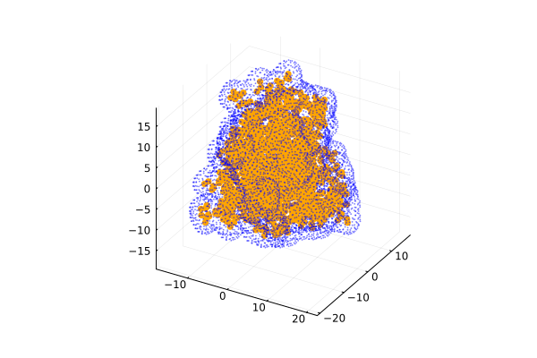
In some situations, it might be useful to visualize the surface. The dots that form the surface can be obtained by running sasa_particles with the output_dots option set to true. Here, we use fewer dots for better visualization:

atom_sasa = sasa_particles(prot; n_dots=100, output_dots=true)

SASA{StandardAtomicRadii, 3, Vector{Atom{Nothing}}}
    Number of particles: 1463
    Total SASA: 5342.6265
    Output of dots: true 

Where the atom_sasa.dots field contains the dots that are accessible to the surface for each atom. These can be plotted, for example, with:

using Plots
dots = reduce(vcat, atom_sasa.dots)
scatter(Tuple.(positions(prot)); color=:orange, msw=0, label="") # atom coordinates
scatter!(Tuple.(dots); # surface dots
    color=:blue, ms=1, msw=0, ma=0.5, # marker properties
    label="",
)

SIRAH solvent accessible area

To compute the solvent accessible surface area of SIRAH models, call the sasa_particles(SIRAH, ...) method, after loading the custom protein residues and elements of the SIRAH force field:

using PDBTools
custom_protein_residues!(SIRAH)
custom_elements!(SIRAH)
sirah_pdb = read_pdb(PDBTools.SIRAHPDB)

   Vector{Atom{Nothing}} with 22 atoms with fields:
   index name resname chain   resnum  residue        x        y        z occup  beta model segname index_pdb
       1   GN      sI     A        1        1  161.582  517.490  112.440  0.00  0.00     1       A         1
       2   GC      sI     A        1        1  160.232  516.820  112.280  0.00  0.00     1       A         2
⋮
      21   GC      sG     A        5        5  156.642  505.730  109.530  0.00  0.00     1       A        21
      22   GO      sG     A        5        5  156.002  505.070  111.770  0.00  0.00     1       A        22

Now we compute the SASA of the full structure:

s_sirah = sasa_particles(SIRAH, sirah_pdb)

SASA{CustomAtomicRadii, 3, Vector{Atom{Nothing}}}
    Number of particles: 22
    Total SASA: 1535.7573
    Output of dots: false 

And the SASA of subsets of the structure can also be obtained:

sasa(s_sirah, "sidechain")

812.94617f0

Here we remove the custom elements and residues, to guarantee proper execution of test codes:

remove_custom_protein_residues!()
remove_custom_elements!()

Dict{String, PDBTools.Element} with 267 entries:
  "He"        => Element(:He, String15("He"), "Helium", 2, 4.0026, false, 1.4)
  "Cd"        => Element(:Cd, String15("Cd"), "Cadmium", 48, 112.41, false, 1.58)
  "Ruthenium" => Element(:Ru, String15("Ru"), "Ruthenium", 44, 101.07, false, NaN)
  "Ge"        => Element(:Ge, String15("Ge"), "Germanium", 32, 72.59, false, 2.11)
  "Fr"        => Element(:Fr, String15("Fr"), "Francium", 87, 223.0, false, 3.48)
  ⋮           => ⋮

Save and load SASA objects

The SASA object can be stored in a file, something that can be useful for very large systems.

save(filename::AbstractString, s::SASA)

load(SASA, filename::String)

outfile = tempname() * ".json"
save(outfile, atom_sasa)
atom_sasa_loaded = load(SASA, outfile)

SASA{StandardAtomicRadii, 3, Vector{Atom{Nothing}}}
    Number of particles: 1463
    Total SASA: 5342.6265
    Output of dots: true 

The file stores the radii model used in the original calculation, so the loaded object preserves the type parameter:

typeof(atom_sasa)

SASA{StandardAtomicRadii, 3, Vector{Atom{Nothing}}}

typeof(atom_sasa_loaded)

SASA{StandardAtomicRadii, 3, Vector{Atom{Nothing}}}

The same works for alternative radii models, such as CreamerUnitedAtomRadii:

atom_sasa_creamer = sasa_particles(CreamerUnitedAtomRadii, prot)
save(outfile, atom_sasa_creamer)
atom_sasa_creamer_loaded = load(SASA, outfile)
typeof(atom_sasa_creamer_loaded)

SASA{CreamerUnitedAtomRadii, 3, Vector{Atom{Nothing}}}

Richards' radii

This parameterization uses the classic united-atom radii of Richards (1977) and Richmond & Richards (1978), assigning each heavy atom to a group (tetrahedral/sp3 or trigonal/sp2 carbon, nitrogen, or oxygen, plus thiol or thioether sulfur) based on the same hybridization classification used for the Creamer radii above. Hydrogens are ignored, as in the Creamer parameterization:

atom_sasa_richards = sasa_particles(RichardsUnitedAtomRadii, prot)
sasa(atom_sasa_richards)

5234.202f0

Two alternative radii sets, both taken from the same source table, are available through the radii_set keyword:

sasa(sasa_particles(RichardsUnitedAtomRadii, prot; radii_set=:set2)) # Richmond & Richards, 1978 (default)

5234.202f0

sasa(sasa_particles(RichardsUnitedAtomRadii, prot; radii_set=:set1)) # Richards, 1977

5268.6494f0

This parameterization reproduces the SASA calculations of SurfaceRacer (Tsodikov, Record & Sergeev) with a mean absolute error of about 2%.

Excluding solvent-sealed cavities

The problem

sasa_particles implements the Shrake-Rupley algorithm: for each atom, a set of points ("dots") is placed on a sphere of radius atom_radius + probe_radius, and a dot counts toward that atom's SASA if it is not covered by any other single atom's inflated sphere. This is a purely local, pairwise test – the same category of algorithm used by, e.g., GROMACS's gmx sasa (an Eisenhaber et al. 1995 "double cubic lattice" variant of Shrake-Rupley) and VMD's measure sasa – and it has no notion of whether a dot that survives it is actually connected to bulk solvent by some continuous path, or whether it instead sits on the wall of a fully sealed interior cavity. For most protein structures the resulting error is small (a fraction of a percent to a couple of percent of the total SASA), because most proteins don't have much topologically sealed interior void space, but it is not zero, and it is exactly the distinction that some reference programs – notably SurfaceRacer – do make (they compute "outside", i.e. solvent-connected, ASA as topologically distinct from interior-cavity ASA, and exclude the latter).

The algorithm

sasa_particles(...; exclude_cavities=true) adds exactly that distinction, as a post-processing step on top of the ordinary Shrake-Rupley result. It works directly on the dots the pairwise test already found exposed – not on a separate, discretized voxel/grid representation of the structure (an earlier version of this feature did use a voxel grid; it was abandoned because it was both less accurate and far more sensitive to its own tuning parameters, for reasons described in cavity_exclusion.jl's module docstring):

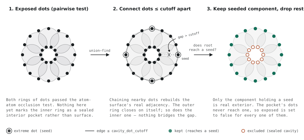
1. Collect every exposed dot of every atom into a single point cloud, in absolute (not atom-relative) coordinates.
2. Connect two dots, via a union-find structure, whenever they are within cavity_dot_cutoff of each other in 3D space. This reconstructs the adjacency of the real, continuous molecular surface directly from the already- computed dot cloud, rather than from a resampled grid.
3. Seed an "exterior" component with the (up to six) dots that individually maximize or minimize each Cartesian coordinate (x, y, z) of the whole structure. Each of these is, by construction, on the true convex, solvent-exposed exterior of the structure; using six independent seeds (rather than a single one) protects against any one of them landing, by coincidence, in a small disconnected sliver.
4. Exclude any exposed dot whose connected component does not contain one of these seeds – i.e., any dot that is only reachable from other exposed dots that are themselves sealed off from the true exterior.

The figure below sketches the mechanism on a cross-section of a ring of atoms sealing a small central cavity. Both the outer surface and the cavity wall carry exposed dots after step 1 ("Collect"), indistinguishable from each other; step 2 ("Connect") reconstructs two disconnected rings, since the gap across the cavity is wider than cavity_dot_cutoff; step 3/4 ("Seed" / "Exclude") keep only the ring reachable from a seed and clear the other:

This only ever removes area that the plain pairwise test already counted; it never adds any, and it has no notion of periodic boundary conditions (exclude_cavities=true together with a non-nothing unitcell raises an error).

cavity_dot_cutoff defaults to twice the estimated nearest-neighbor spacing between dots on the largest inflated atom sphere present (which depends on n_dots and the atom radii/probe radius in use), but the result is essentially insensitive to the exact multiple over a wide range: on the 3CNA tetramer/dimer benchmark used in this package's tests, cutoffs from 0.6 to 1.3 Å (for the default n_dots=512) all agree to better than 0.01%. This robustness is the main advantage over the abandoned voxel-grid approach, whose result changed non-monotonically – and sometimes drastically – with its own tuning parameters (see cavity_exclusion.jl for the full comparison).

dimer = read_pdb(PDBTools.DIMERPDB)
sasa(sasa_particles(dimer))                            # default: no cavity exclusion

12462.061f0

sasa(sasa_particles(dimer; exclude_cavities=true))     # with cavity exclusion

12049.638f0

Scope and limitations

This is a compatibility feature for reproducing SurfaceRacer's specific ASA convention – not a general correctness fix, and not a claim that the plain Shrake-Rupley default is "wrong" (it isn't; it's the same convention used by GROMACS and VMD). It matters here because it is the convention some transfer-model parameterizations (see the Record model) were calibrated against. Two caveats worth keeping in mind:

• It is an approximation, not a bit-for-bit reproduction of SurfaceRacer's own exact analytical algorithm. On the 3CNA benchmark, it recovers the difference between two structures' SASA (the quantity that enters an m-value) to within about 1% of SurfaceRacer's own number, but individual absolute SASA totals can still be off by a percent or two.
• Genuinely small compounds (individual amino acids, short peptides, sugars, and similar) have essentially no topologically sealed interior void space to begin with, so exclude_cavities has little to no effect on them; the correction only becomes appreciable for folded domains and, especially, for buried protein-protein or subunit-subunit interfaces.