MolecularMinimumDistances

MolecularMinimumDistancs.jl computes the minimum distance between molecules, which are represented as arrays of coordinates in two or three dimensions.

To understand the utility and purpose of this package, consider the image below:

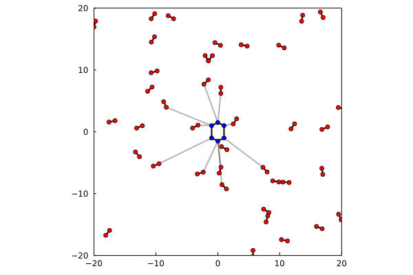
Here, there is one blue molecule, with 6 atoms, and several red molecules, with 2 atoms each. The package has identified which are the molecules of the red set that have at leat one atom within a cutoff from the atoms of the blue molecule, and annotated the corresponding atoms and the distances.

Features

Fast cell-list approach, to compute minimum-distance for thousands, or millions of atoms.
General periodic boundary conditions supported.
Advanced mode for in-place calculations, for non-allocating iterative calls (for analysis of MD trajectories, for example).
Modes for the calculation of minimum-distances in sets of molecules.

Most typical use: Understanding solvation

This package was designed as the backend for computing minimum distance distribution functions, which are useful for understanding solute-solvent interactions when the molecules have complex shapes.

The most typical scenario is that of a protein, or another macromolecule, in a box of solvent. For example, here we download a frame of a protein which was simulated in a mixture of water and TMAO:

julia> using PDBTools

julia> system = MolecularMinimumDistances.download_example()
   Array{Atoms,1} with 62026 atoms with fields:
   index name resname chain   resnum  residue        x        y        z  beta occup model segname index_pdb
       1    N     ALA     A        1        1   -9.229  -14.861   -5.481  0.00  1.00     1    PROT         1
       2  HT1     ALA     A        1        1  -10.048  -15.427   -5.569  0.00  0.00     1    PROT         2
       3  HT2     ALA     A        1        1   -9.488  -13.913   -5.295  0.00  0.00     1    PROT         3
                                                       ⋮ 
   62024  OH2    TIP3     C     9339    19638   13.485   -4.534  -34.438  0.00  1.00     1    WAT2     62024
   62025   H1    TIP3     C     9339    19638   13.218   -3.647  -34.453  0.00  1.00     1    WAT2     62025
   62026   H2    TIP3     C     9339    19638   12.618   -4.977  -34.303  0.00  1.00     1    WAT2     62026

Next, we extract the protein coordinates, and the TMAO coordinates:

julia> protein = coor(system,"protein")
1463-element Vector{SVector{3, Float64}}:
 [-9.229, -14.861, -5.481]
 [-10.048, -15.427, -5.569]
 [-9.488, -13.913, -5.295]
 ⋮
 [6.408, -12.034, -8.343]
 [6.017, -10.967, -9.713]

julia> tmao = coor(system,"resname TMAO")
2534-element Vector{SVector{3, Float64}}:
 [-23.532, -9.347, 19.545]
 [-23.567, -7.907, 19.381]
 [-22.498, -9.702, 20.497]
 ⋮
 [13.564, -16.517, 12.419]
 [12.4, -17.811, 12.052]

The system was simulated with periodic boundary conditions, with sides in this frame of [83.115, 83.044, 83.063], and this information will be provided to the minimum-distance computation.

Finally, we find all the TMAO molecules having at least one atom closer than 12 Angstroms to the protein, using the current package (TMAO has 14 atoms):

julia> list = minimum_distances(
           xpositions=tmao, # solvent
           ypositions=protein, # solute
           xn_atoms_per_molecule=14,
           cutoff=12.0,
           unitcell=[83.115, 83.044, 83.063]
       )
181-element Vector{MinimumDistance{Float64}}:
 MinimumDistance{Float64}(false, 0, 0, Inf)
 MinimumDistance{Float64}(false, 0, 0, Inf)
 ⋮
 MinimumDistance{Float64}(true, 2526, 97, 9.652277658666891)

julia> count(x -> x.within_cutoff, list)
33

Thus, 33 TMAO molecules are within the cutoff distance from the protein, and the distances can be used to study the solvation of the protein.

Performance

This package exists because this computation is fast. For example, let us choose the water molecules instead, and benchmark the time required to compute this set of distances:

julia> water = coor(system,"resname TIP3")
58014-element Vector{SVector{3, Float64}}:
 [-28.223, 19.92, -27.748]
 [-27.453, 20.358, -27.476]
 [-27.834, 19.111, -28.148]
 ⋮
 [13.218, -3.647, -34.453]
 [12.618, -4.977, -34.303]

julia> using BenchmarkTools

julia> @btime minimum_distances(
           xpositions=$water, # solvent
           ypositions=$protein, # solute
           xn_atoms_per_molecule=3,
           cutoff=12.0,
           unitcell=[83.115, 83.044, 83.063]
       );
  6.288 ms (3856 allocations: 13.03 MiB)

To compare, a naive algorithm to compute the same thing takes roughly 400x more for this system size:

julia> @btime MolecularMinimumDistances.naive_md($water, $protein, 3, [83.115, 83.044, 83.063], 12.0);
  2.488 s (97 allocations: 609.16 KiB)

And the computation can be made faster and in-place using the more advanced interface that allows preallocation of main necessary arrays:

julia> sys = CrossPairs(
           xpositions=water, # solvent
           ypositions=protein, # solute
           xn_atoms_per_molecule=3,
           cutoff=12.0,
           unitcell=[83.115, 83.044, 83.063]
       )
CrossPairs system with:

Number of atoms of set: 58014
Number of atoms of target structure: 1463
Cutoff: 12.0
unitcell: [83.12, 0.0, 0.0, 0.0, 83.04, 0.0, 0.0, 0.0, 83.06]
Number of molecules in set: 4144

julia> @btime minimum_distances!($sys);
  2.969 ms (196 allocations: 22.80 KiB)

The remaining allocations occur only for the launching of multiple threads:

julia> sys = CrossPairs(
           xpositions=water, # solvent
           ypositions=protein, # solute
           xn_atoms_per_molecule=14,
           cutoff=12.0,
           unitcell=[83.115, 83.044, 83.063],
           parallel=false # default is true
       );

julia> @btime minimum_distances!($sys);
  15.249 ms (0 allocations: 0 bytes)

Details of the illustration

The initial illustration here consists of a toy solute-solvent example, where the solute is an approximately hexagonal molecule, and the solvent is composed by 40 diatomic molecules. The toy system is built as follows:

using MolecularMinimumDistances, StaticArrays
# x will contain the "solvent", composed by 40 diatomic molecules
T = SVector{2,Float64}
x = T[]
cmin = T(-20,-20)
for i in 1:40
    v = cmin .+ 40*rand(T)
    push!(x, v)
    theta = 2pi*rand()
    push!(x, v .+ T(sin(theta),cos(theta)))
end
# y will contain the "solute", composed by an approximate hexagonal molecule
y = [ T(1,1), T(1,-1), T(0,-1.5), T(-1,-1), T(-1,1), T(0,1.5) ]

Next, we compute the minimum distances between each molecule of x (the solvent) and the solute. In the input we need to specify the number of atoms of each molecule in x, and the cutoff up to which we want the distances to be computed:

julia> list = minimum_distances(
           xpositions=x,
           ypositions=y,
           xn_atoms_per_molecule=2,
           unitcell=[40.0, 40.0],
           cutoff=10.0
       )
40-element Vector{MinimumDistance{Float64}}:
 MinimumDistance{Float64}(true, 2, 3, 1.0764931248364737)
 MinimumDistance{Float64}(false, 0, 0, Inf)
 MinimumDistance{Float64}(false, 0, 0, Inf)
 ⋮
 MinimumDistance{Float64}(true, 74, 5, 7.899981412729262)
 MinimumDistance{Float64}(false, 0, 0, Inf)

The output is a list of MinimumDistance data structures, one for each molecule in x. The true indicates that a distance smaller than the cutoff was found, and for these the indexes of the atoms in x and y associated are reported, along with the distance between them.

In this example, from the 40 molecules of x, eleven had atoms closer than the cutoff to some atom of y:

julia> count(x -> x.within_cutoff, list)
11

We have an auxiliary function to plot the result, in this case where the "atoms" are bi-dimensional:

using Plots
import MolecularMinimumDistances: plot_md!
p = plot(lims=(-20,20),framestyle=:box,grid=false,aspect_ratio=1)
plot_md!(p, x, 2, y, 6, list, y_cycle=true)

will produce the illustration plot above, in which the nearest point between the two sets is identified.