Microcanonical Molecular Dynamics Simulation

Open the file md-simple.jl, which contains the simulation algorithm. The simulation starts with random velocities, adjusted to the desired thermodynamic average of 0.6 units/atom ($kT=0.6$ in a two-dimensional system). We will call this average kinetic energy "temperature". The integration algorithm is Velocity-Verlet, which consists of propagating the positions with

\[\vec{x}(t+\Delta t) = \vec{x}(t) + \vec{v}(t)\Delta t + \frac{1}{2}\vec{a}(t)\Delta t^2\]

where $\vec{a}(t)=\vec{F}(t)/m$, and $\vec{F}(t)$ is the force at the current time. The force is then computed at the next time step with

\[\vec{F}(t+\Delta t) = -\nabla V\left[\vec{x}(t)\right]\]

and then the velocities at the next instant are computed with

\[\vec{v}(t+\Delta t) = \vec{v}(t) + \frac{1}{2}\left[ \frac{\vec{F}(t)}{m}+\frac{\vec{F}(t+\Delta t)}{m}\right]\]

completing the cycle. In this example, masses are taken to be unity for simplicity. The simulation is run for nsteps steps, with integration time step $\Delta t$, which is an input parameter, dt, defined in Options.

The simulation has no temperature or pressure control. It is a propagation of the trajectory according to Newton's laws, which should conserve energy. This is called a "microcanonical" or "NVE" simulation (conserving, in principle, the number of particles, the volume, and the total energy).

3.1. Integration time step

To perform a simple MD with an integration time step of dt=1.0, run:

julia> out = md(sys,Options(dt=0.1));

In principle, 2000 integration steps of the equations of motion are expected to be performed. Try integration time steps between 1.0 and 0.01. Note what happens to the energy. Note what happens to the average kinetic energy, which was initialized at 0.6 units/atom. Discuss the choice of integration time step and the kinetic energy values obtained. The simulations that follow will use an integration time step dt = 0.05.

It is possible to control the print frequency and the number of points saved to the trajectory file with the iprint and iprintxyz options:

julia> out = md(sys,Options(dt=0.1,iprint=1,iprintxyz=5))

The total number of steps is controlled with the nsteps parameter.

The out variable returned from the simulation is a matrix with the energies and temperature at each simulation step. The simulation will likely "explode" with large time steps. To visualize this, we can do:

julia> using Plots

julia> plot(
          out,ylim=[-100,100],
          label=["Potential" "Kinetic" "Total" "Temperature"],
          xlabel="step"
       )

And we will obtain a plot similar to:

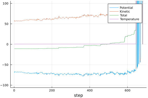
For smaller time steps the simulation should be able to run to completion. We can view the result again, and it should look something like:

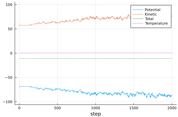
Observe and try to understand the amplitudes of the oscillations of the kinetic and potential energies, and the amplitudes of the oscillations of the total energy. What causes each of the oscillations? Observe how these oscillations depend on the integration time step.

3.2. Trajectory visualization

Finally, open the trajectory using VMD. It is not necessary to exit the Julia session. By pressing ; (semicolon), a shell> prompt will appear, from which VMD can be run, if it is correctly installed and available on the path:

shell> vmd traj.xyz

Within VMD, choose the VDW representation under

Graphics -> Representations -> Drawing Method -> VDW

and run the command

vmd> pbc set { 100. 100. 100. } -all

to indicate the periodicity of the system. To explicitly represent the periodic system, select +X;+Y;-X;-Y under

Graphics -> Representations -> Periodic

To exit VMD use the exit command, and to return to the Julia prompt from shell>, use backspace.

3.3. Complete summary code

using FundamentosDMC, Plots

sys = System(n=100)
minimize!(sys)
out = md(sys,Options(dt=0.05))

plot(out,ylim=[-100,100],
    label=["Potential" "Kinetic" "Total" "Temperature"],
    xlabel="step"
)

The file traj.xyz is generated and can be visualized in VMD.